Data structures for computational statistics klinke 1997 05 20
Bạn đang xem bản rút gọn của tài liệu. Xem và tải ngay bản đầy đủ của tài liệu tại đây (7 MB, 286 trang )
Contributions to Statistics
V. FedorovIW.G. Milller/I.N. Vuchkov (Eds.) Model-Oriented Data Analysis,
XIIl248 pages, 1992
J. Antoch (Ed.) Computational Aspects of Model Choice,
VII1285 pages, 1993
W.G. MIDlerIH.P. Wynn/A.A. Zhigljavsky (Eds.)
Model-Oriented Data Analysis,
X1III287 pages, 1993
P. MandllM. HuSkov' (Eds.)
Asymptotic Statistics
Xl474 pages, 1994
P. DirschedllR. Ostermann (Eds.)
Computational Statistics
VIY553 pages, 1994
C.P. KitsosIW.G. Milller (Eds.)
MODA4 - Advances in Model-Oriented Data Analysis,
XlV1297 pages, 1995
H. Schmidli
Reduced Rank Regression,
Xl179 pages, 1995
W. HllrdIeIM. G. Schimek (Eds.)
Statistical Theory and Computational Aspects of Smoothing,
VIDn65 pages, 1996
Sigbert Klinke
Data Structures for
Computational Statistics
With 108 Figures
and 43 Tables
Springer-Verlag Berlin Heidelberg GmbH
Series Editors
Wemer A. Miiller
Peter Schuster
Author
Dr. Sigbert Klinke
Humboldt-University of Berlin
DeprunnentofEconomics
Institute of Statistics and Econometrics
Spandauer Str. 1
D-10178 Berlin, Germany
ISBN 978-3-7908-0982-4
Cataloging-in-Publication Data applied for
Die Deutsche 8ibliothek - CIP-Einheitsaufnahme
Klinke, Sigbert: Data sttuctures for computational statistics: with 43 tables / Sigbert Klinke. Heidelberg: Physica-VerI., 1997
(Conbibutions to statistics)
ISBN 978-3-7908-0982-4
ISBN 978-3-642-59242-3 (eBook)
DOI 10.1007/978-3-642-59242-3
This work is subject to copyright AII rights are reserved, whether the whole or prut of the material
is concemed, specifical1y the rights of translation, reprinting, reuse of iIIustrations, recitation, broadcasting, reproduction on microfilm or in any other way, and storage in data banks. Duplication of
this publication or parts thereof is permitted only under the provisions of the German Copyright
Law of September 9, 1965, in its current version, and permission for use must always be obtained
from Physica-Verlag. Violations are Iiable for prosecution under the German Copyright Law.
© Springer-Verlag Berlin Heidelberg 1997
OriginaIly published by Physica-Verlag Heidelberg in 1997
The use of general descriptive names, registered names, trademarks, etc. in this publication does not
imply, even in the absence of a specific statement, that such names are exempt from the relevant
protective laws and regulations and therefore free for general use.
Softcover Design: Erich Kirchner, Heidelberg
SPIN 10558916
88/2202-5 4 3 2 1 0- Printed on acid-free paper
Preface
Since the beginning of the seventies computer hardware is available to use
programmable computers for various tasks. During the nineties the hardware
has developed from the big main frames to personal workstations. Nowadays
it is not only the hardware which is much more powerful, but workstations can
do much more work than a main frame, compared to the seventies. In parallel
we find a specialization in the software. Languages like COBOL for businessorientated programming or Fortran for scientific computing only marked the
beginning. The introduction of personal computers in the eighties gave new
impulses for even further development, already at the beginning of the seventies some special languages like SAS or SPSS were available for statisticians.
Now that personal computers have become very popular the number of programs start to explode. Today we will find a wide variety of programs for
almost any statistical purpose (Koch & Haag 1995).
The past twenty years of software development have brought along a great
improvement of statistical software as well. It is quite obvious that statisticians have very specific requirements for their software. There are two developments in the recent years which I regard as very important. They are
represented by two programs:
• the idea of object orientation which is carried over from computer science and realized in S-Plus
• the idea of linking (objects) is present since the first interactive statistical program (PRIM-9). In programs like DataDesk, X-Lisp-Stat or
Voyager this idea has reached its most advanced form. Interactivity has
become an important tool in software (e.g. in teachware like CIT) and
statistics.
The aim of this thesis is to discuss and develop data structures which are
necessary for an interface of statistics and computing. Naturally the final
aim will be to build powerful tools so that statisticians are able to work
efficiently, meaning a minimum use of computing time.
Before the reader will read the details, I will use the opportunity to express
my gratefulness to all the people who helped me and joined my way. At the
first place is, Prof. Dr. W. HardIe. Since 1988 when I started to work as a
student for him he guided me to the topic of my thesis. The development
of XploRe 2.0, where I had only a small participation, and XploRe 3.0 to
3.2 gave me a lot of insights in the problems of statistical computing. With
vi
Preface
his help I got a grant from the European Community, which brought me to
Louvain-Ia-Neuve and to my second Ph.D.-advisor, Prof. Dr. L. Simar.
A lot of people from CORE have contributed to the accomplishment of my
work. I would like to mention Heraclis Polemarchakis, Luc Bauwens and
Sheila Verkaeren. I am very thankful to the staff of the "Institut de Statistique" for their support and help, especially Leopold Simar, Alois Kneip,
Irene Gijbels and Alexander Tsybakov. The atmosphere of Louvain-Ia-Neuve
was very inspiring for my work. I have to mention the conference about "Statistical Computing" hold in Reisensburg because it gave me an insight in a
lot of practical problems which have enriched my thesis.
I have also to thank a lot offriends and colleagues for their help and company:
Isabel Proenca, Margret Braun, Berwin Turlach, Sabine Dick, Janet Grassmann, Marco and Maria Bianchi, Dianne Cook, Horst and Irene BertschekEntorf, Dirk and Kristine Tasche, Alain Desdoigt, Cinzia Rovesti, Christian Weiner, Christian Ritter, Jorg Polzehl, Swetlana Schmelzer, Michael
Neumann, Stefan Sperlich, Hans-Joachim Mucha, Thomas Kotter, Christian
Hafner, Peter Connard, Juan Rodriguez, Marlene Miiller and of course my
family.
I am very grateful for the financial support of the Deutsche Forschungsgemeinschaft (DFG) through the SFB 373 "Quantifikation und Simulation
okonomischer Prozesse" at the Humboldt University of Berlin which makes
the publication of my thesis possible.
Contents
1
2
Introduction
1
1.1 Motivation
1
1.2 The Need of Interactive Environments
4
1.3 Modern Computer Soft- and Hardware .
18
Exploratory Statistical Techniques
25
2.1
25
Descriptive Statistics .
2.2 Some Stratifications
28
2.3 Boxplots . . . . . . .
29
2.4 Quantile-Quantile Plot .
31
2.5 Histograms, Regressograms and Charts.
33
...
40
2.7 Scatterplot Matrices
46
2.8 Three Dimensional Plots .
48
2.9 Higher Dimensional Plots
52
2.10 Basic Properties for Graphical Windows
58
Some Statistical Applications.
61
3.1 Cluster Analysis
61
3.2 Teachware . . . .
69
3.3 Regression Methods
72
Exploratory Projection Pursuit
91
2.6 Bivariate Plots
3
4
4.1
Motivation and History
....
91
4.2 The Basis of Exploratory Projection Pursuit .
102
4.3 Application to the Swiss Banknote Dataset
145
4.4 Multivariate Exploratory Projection Pursuit.
148
viii
5
6
Contents
4.5
Discrete Exploratory Projection Pursuit . . . . . . . . . . ..
162
4.6
Requirements for a Tool Doing Exploratory Projection Pursuit 166
Data Structures . . . . .
169
5.1
For Graphical Objects
169
5.2
For Data Objects
173
5.3
For Linking . . .
181
5.4
Existing Computational Environments
187
Implementation in XploRe . . .
197
6.1
Data Structures in XploRe 3.2
197
6.2
Selected Commands in XploRe 3.2
210
6.3
Selected Tools in XploRe 3.2
217
6.4
Data Structure in XploRe 4.0
233
6.5
Commands and Macros in XploRe 4.0
237
7 Conclusion
239
A The Datasets .......
241
A.1 Boston Housing Data.
241
A.2 Berlin Housing Data and Berlin Flat Data .
242
A.3 Swiss Banknote Data .
245
......
245
A.4 Other Data
B Mean Squared Error of the Friedman-Tukey Index ..... 247
C Density Estimation on Hexagonal Bins
257
D Programs . . . . . . .
263
D.1 XpioRe Programs.
263
D.2 Mathematica Program
266
E Tables
...
269
References .
277
1
Introduction
Summary
This chapter first explains what data structures are and why they are important for statistical software. Then we take a look at why we need interactive
environments for our work and what the appropriate tools should be. We do
not discuss the requirements for the graphical user interface (G UI) in detail.
The last section will present the actual state of soft- and hardware and which
future developments we expect.
1.1
Motivation
What are data structures ?
The term "Data Structures" describes the way how data and their relationships are handled by statistical software. Data does not only mean data in
the common form like matrices, arrays etc, but also graphical data (displays,
windows, dataparts) and the links between all these data. This also influences
the appearance of a programming language and we have to analyze this to
some extent too.
Why examining data structures ?
In statistical software we have to distinguish between two types of programs:
programs which can be extended and programs which only allow what the
programmer had intended. In order to extend the functionality of the programs of the first class we would need a programming language which can not
be recognized by the user (e.g. visual programming languages). This is important for statistical research, if we want to develop new computing methods
for statistical problems.
We have a lot of successful statistical software available, like SAS, BDMP, SPSS,
GAUSS, S-Plus and many more. Mostly the data structure is developed ad
hoc, and the developers have to make big efforts to integrate new developments from statistics and computer science. Examples are the inclusion of the
Trellis display or the linking facilities in S-Plus or the interactive graphics
in SAS.
2
Introduction
Therefore it seems necessary to decompose the tools of a statistical program
(graphics, methods, interface) and to see which needs statisticians have and
to develop and implement structures which in some sense will be general for
all statistical programs.
Nevertheless some decisions are depending on the power of the underlying
hardware. These will be revised as soon as the power of the hardware increases.
The programs of the second class can hide their structures. An analysis of
these programs will be very difficult. We can only try to analyze the data
structure by their abilities and their behaviour.
What is my contribution?
We first examine the needs in graphics, linking and data handling in extendable statistical software. The next step is to develop data structures that
allow us to satisfy the needs as well as possible. Finally we describe our implementation of the data structures. There was a discrepancy between our
ideas and the implementation in XploRe 3.2, partly due to the fact that this
implementation exists longer than my thesis, but we also had some technical limitations from the side of the hard- and software. For example, in the
beginning we had a 640 KB-limit of the main memory and we did not use
Windows 3.1 in XploRe 3.2. In XploRe 4.0, under UNIX, we will implement
our ideas in a better way, but we are still at the beginning of the development.
A extendable statistical software is composed of three components:
• the graphical user interface (G UI)
In the first chapter we discuss the GUI shortly regarding why we need
interactive programmable environments.
• the statistical graphic
The graphics have to fulfill certain goals: there are statistical graphical
methods and we need to represent the results of our analysises. So in
chapter 2 we examine statistical graphics, in chapter 3 and 4 complete
statistical methods (exploratory projection pursuit, cluster analysis)
will be discussed.
• the statistical methods
The statistical methods are often difficult to separate from the graphics
(e.g. grand tour, exploratory projection pursuit). However we can decompose graphical objects into a mathematical computation and into
a visualization step. We show this in the beginning of chapter 5. Another aspect of statistical methods is the deepness of the programming
language. The deepness for regression methods is discussed in detail in
the last section of chapter 4.
Introduction
3
Part of the programming language is also the handling of data objects. In
chapter 5 we give two examples (local polynomial regression, exploratory
projection pursuit) why matrices are not sufficient for data handling. The
use of arrays has consequences for the commands and the operators in a
programming language. The need for hierarchical objects to store different
objects and metadata also has an impact on commands and operators.
The question of linking data objects (data matrices, graphical objects etc.)
is also part of chapter 5. The last chapter describes the implementation in
the software XploRe. In XploRe 3.2, a program which runs under DOS, we
have implemented the data structures of graphics and linking. In XploRe 4.0,
which currently runs under UNIX and Motif, we have implemented arrays.
Where are the difficulties ?
The implementation phase of XploRe 3.2 lasted of course more than two years.
The main problem at the beginning was that I did not have any idea which
needs a statistician has. Nevertheless the decision about the data structures
had to be made in an early phase of the implementation. Each missdecision
I made had to be corrected later with an enormous amount of work. Some
examples are:
• the programming language
When I developed the programming language my aim was to build a
language which simplifies matrix manipulations, but I did not want to
develop a whole language with loops, selections etc. So I chose to build
an interpreter which makes the XploRe language slow. Especially loops
which interpret each line again and again instead of interpreting it once
by using a compact code are very slow.
• the basic datatype
For a matrix of numbers I chose the 4-byte float numbers as a basic
datatype. Since in the beginning we had a technical limitation under
DOS with max. 640 KB RAM, we wanted to store float numbers as
short as possible. Since the compiled program already needs 400 KB
memory we were only able to handle small datasets. Later I figured
out that for some computations the precision was not high enough, so
I changed to 8-byte float numbers. It took me some months to get the
program to run properly afterwards.
• linking and brushing
The implementation of linking and brushing in XploRe allows only transient brushing. This is due to the data structure I chose. After recognizing this I decided it was not worthwhile implementing a structure
which allows nontransient brushing in XploRe 3.2. With an additional
structure this would be possible, and we will correct this decision in
XploRe 4.0.
4
Introduction
The data structure I present in chapter 5 appeared only after I had thought
about the needs. In fact it was a process of trying and learning. When Isabel Proenca implemented the teachware macros I saw that we needed programmable menus. So I implemented the command MEIU which works in a
window. One problem is that the cursor was supposed to change from an
arrow to a bar. But after printing a display with <Ctrl-p> the cursor again
appeared as an arrow. Only after the next movement it would appear as bar
again. Another problem appeared when printing the <F3>-box together with
boxplots. The standard behaviour was that the box disappeared from the
screen and reappeared after printing, but did not appear in the printout. It
took me nearly a week to change this behaviour.
Nevertheless I believe that I could build an efficient system. The development
of most of the tools took me only one day or two. Of course the fine tuning
like linking and everything appearing in the right time and the right place
often took much more time. The wavelet regression macro is an example for
this: the development was done in one day, but for the final form I needed
more than a week. Additionally to the inclusion of the threshold method
suggested by Michael Neumann I had to modify the commands handling the
wavelet computations.
The analysis of data structures in other programs is very difficult. Since most
them are commercial products I have no access to the source codes. Only
from the way how the user sees these programs I can try to guess which data
structures are used. Dynamic graphics and linking seems to be a real problem
in S-Plus (e.g. there is practically no possibility for printing the scatterplot
matrix). New tools like the Trellis display or linking require a quite extended
reprogramming of these languages. So I only give a short overview of the
facilities of the different programs.
Another problem was that I needed an overview about a lot of different
statistical techniques, and I needed knowledge about the implementation of
these techniques rather than the statistical and theoretical properties.
Some interesting problem, e.g. the treatment of missings or the error handling, could not be handled in a proper way because of a lack of time.
1.2 The Need of Interactive Environments
1.2.1
Why Interactivity ?
As soon as interactive graphical terminals were available statisticians start
to use them. In 1974, Fisherkeller, Friedman & Tukey (1988) developed a
program called PRIM-9, which allowed analyzing a dataset of up to nine
Introduction
5
dimensions interactively. They implemented the first form of linking, e.g. they
allowed to mask out datapoints in one dimension such that all datapoints
above or below a certain value would not be drawn. In a scatterplot which
shows two different variables of the dataset the according datapoints would
also not be drawn. They showed (with an artificial dataset) that this can lead
to new insights about the dataset.
The computational equipment which was used in the seventies to run PRIM-9
was expensive. Nowadays computer power has improved and a lot of programs
offer the facilities of PRIM-9. Nevertheless the idea of interactive environments
needs time to become a standard tool in statistics.
In batch programming as it was common during the sixties and seventies,
a statistical analysis needed a lot of time. There were two possibilities to
work: step by step, which consumes a lot of time, or to write big programs
which compute everything. The programming environment SAS, a program
available already for a long time, computes a lot of superfluous informations
although we may be interested just in the regression coefficients. As an example we show the regression of the variable FA (area of a flat in square meter)
against FP (the price per flat in thousand DM) of the Berlin flat data; for a
description of the dataset see section A. Figure 1.1 shows the SAS-output for
a linear regression.
Figure 1.2 is an indicator of the analysis on the run, which shows that the
linear regression (y = az + b) is not appropriated for this dataset. Especially
at the ends of the dataset we would expect another behaviour. For the left
end we can see this from the coefficients (a'" 5, b "" -67), which tells us we
would even get money for a flat with less than 13 m 2 if we wanted to buy it.
A typical behaviour is to use log( F P) instead of F P. So we can use, as in
this example, the interactive graphics to control the analysis. If we are not
satisfied with the analysis we have to interfere. Here we will have to choose a
nonlinear or nonparametric model. Users also like to control an analysis since
they do not trust computers too much. An example might be that different
statistical programs will give slightly different answers although they perform
the same task (rounding errors, different algorithms).
Interactivity offers to cover "uncertainty" or nonmathematics. Uncertainty
means that we do not know which (smoothing) parameter to choose for a task;
see for example the smoothing parameter selection problem in exploratory
projection pursuit. Often we can simply ask a user for the smoothing parameter, because he has a feeling for the right values for the parameter or can
figure it (interactively) out.
Sometimes it is difficult to represent a visual idea as a mathematical formula. As example serves the selection of a clustering algorithm (hierarchical
methods: the choice of the distance, the choice of the merging method). We
have no general definition of a cluster, and as a consequence we have lot of
6
Introduction
The SAS Systea
17:09 Monday, July 31, 1995
2
Model: MODELl
Dependent Variable: FP
Analysis of Variance
Source
DF
Model
Error
C Total
Root MSE
Dep Mean
C.V.
SUII of
Squares
Mean
Square
F Value
Prob>F
1 61329361.148 61329361.148 4686.772
1365 17861883.086 13085.628635
1366 79191244.234
0.0001
114.39243
357.73167
31.97716
R-square
Adj R-sq
0.7744
0.7743
Parameter Estiaates
Variable DF
INTERCEP
FA
1
1
Paraaeter
Estiaate
Standard
Error
T for HO:
Parameter-O
Prob > ITI
-67.531740
5.429284
6.93971316
0.07930592
-9.731
68.460
0.0001
0.0001
FIGURE 1.1. Output of the linear regression of the variables FA and FP of the
Berlin flat data.
different possibilities to find clusters in the data. Interactivity allows us to
give our expectations into the process of clustering.
Another important advantage of inter activity is that we can "model" sequentially:
• In Figure 1.2 we made a linear regression. In fact we could try a lot of
different regression models. One possibility would be to use nonparametric models; our model might not satisfy the user. Figure 1.4 shows
a robust locally weighted regression. This method tells us something
different about the dataset .
• If we compute the correlation coefficient rxy between the two variables
FA and FP we see in Figure 1.1 that it is '" 0.77. Often programs make
a test immediately afterwards if the coefficient is unequal zero. With
such a large value of the correlation coefficient (n = 1366), no test
Introduction
7
~IUU
111 . 0000000000
3200.0000000000
;;
o
- ..;
:'
0
~
~--~----~~----~----'------r--~
0.5
1.5
1.0
Ar..
2.5
2.0
(·102)
FIGURE 1.2. Output of the linear regression of the variable FA (area of
fiat) and FP (price oUat) ofthe Berlin fiat data (only offers Oct. 1994) .
.
0
w
r.
:
0
'.
~
~
"
"i. :
:
"
0
0
0
0.0
0.2
D.'
Ar. .
0.6
'*10 2 ,
O.B
1.0
FIGURE 1.3. Same picture as Figure 1.2, but focussed in the left lower
corner.
will accept the hypothesis
coefficient is near zero.
rlt:lI
= O. This test only makes sense if the
8
Introduction
Interactivity also allows parallel modeling. For example we can make a linear
and a nonlinear regression on our data, then we can analyze the residuals,
the influence of observations on the fit etc parallel in both methods, e.g. via
linking.
.
.,;
..
..,;
I • • •
'::
"
"
".,;
0.0
0.'
D.'
Ar..
D.'
,*10 2)
0.8
1.0
FIGURE 1.4. Robust locally weighted regression of the variables FP
(price in thousand DM) against FA (area of a flat in square meters).
This estimate coincides better with the feeling that the price should become constant or zero if the area decrease to zero.
1.2.2
The Tools of Interactivity
General
In the last five years the basic operating systems have changed. With the
graphical capabilities available now, the interface of computers have changed
from text based systems (DOS, C-Shell, Korn-Shell, VMS, TSO etc) to graphical interfaces. A lot of computers (MacIntosh, Atari) were developed which
have only graphical interfaces, for other computers graphical interfaces were
developed which sit on top or replace a text based interface (Windows 3.1,
X-Windows, OS/2 2.11). Nowadays even operating systems are available independent of the underlying hardware (Windows NT, NextStep) and we see
a development to unify even the hardware (PowerPC).
The advantage of the window based operating systems is their easiness of
use: instead of having to remember a lot of different commands, we have
just to click the (right) buttons, the menu items and the windows. This is
Introduction
9
a good choice for beginners. Nevertheless a graphical window system is not
always the best choice. Take for example XploRe 2.0, a completely menu
driven program. The data vectors are stored in workspaces. The addition of
two vectors is a complicated task. We have first to click in the menu that
we want to make an addition. Afterwards all possible workspaces are offered
twice to figure out which vectors we want to add. It turns out that a lot of
clicking and moving through menus is necessary, whereas a simple command
like
y
= x [, 1] +x [, 2]
is much easier just to be typed.
The lesson we can learn from this example is that both is necessary: a graphical and a text based interface.
Many ofthe statistical programs overemphasize one ofthe components; DataDesk and XGobi are completely based on graphical interfaces whereas S-Plus,
Mini tab, GAUSS and SAS emphasize too much the text based interface.
The underlying concept of a window system is the one of an office. A desk is
the basis where several folders are spread. Windows represent the different
task we are working on. As a real desk can be overboarded with piles of
papers and books, the window system can have opened too many windows
so that we loose the overview. Especially if the programs do not close their
windows by themselves when inactive the number of windows increases fast.
The size of the screens has become larger and larger: some years ago a 14
inch screen was standard, nowadays more and more computers start with 17
inch screens. This only delays the problem. Another solution which computer
experts offer is a virtual desktop so that we only see a part of the desktop
on the screen. Via mouseclicking or scrolling we can change from one part to
another. Nevertheless a program has to use use intelligent mechanism to pop
up and down windows.
Windows
We need to have different kinds of windows: Windows that allow us to handle
graphics (2D- and 3D-graphics) and windows that handle text(editors, help
systems). It is useful to incorporate text in a picture. In fact in all window
systems we have only graphical windows, but some behave like text windows.
The windows themselves have to perform some basic operations. Stuetzle
(1987) described a system called Plot Windows, which uses a graphical user
interface and proposed some operations:
• A window should to be moved easily to another location.
10
Introduction
• A reshape of a window should be easy.
• Stuetzle wanted to have the possibility of moving windows under a pile
of windows. Today we can iconify a window, that means to close a
window and to place it somewhere as an icon so that we remember
that we have a window. A mouseclick reopens the window.
Displays
XPLORE TWREGEST
HLP$I.1]
_.
a.m..
UP
DICUUII •
•
. . DIe
CIJUOIl III*"
•
Of DIe
:ry
t.!o
X(.1I,1III1(,11,MK[,lJ
INnI.1)
IIAIIWt'I'H H
~JJlC
CROSS-VALIIM.'I'IOII
DIP(.11
5.15000
0.fi5000
12578.325"
1.0
(.to 2]
2.S
CIJUOIl.....
_DIe •
iO
i
i
x
;._.
·.• , .••.••.• ".111 .• 11 ......
FIGURE 1.5. Windows with several informations form a display for a
certain statistical task (here: relationship between the kernel regression
and the selection of the smoothing parameter). A Nadaraya-Watson estimator is used to model the relationship between the variables FA (area
of a flat) and FP (price of a flat).
From my point of view the concept of displays is important in statistics. In
the windows of a display we can show several kinds of information that need
to appear together. As an example see Figure 1.5, which shows a kernel regression on the Berlin flat dataset. The left upper window shows the data
and the fitted line (gray), the right upper window gives us a small help text
that tells us which keys can be used to manipulate the smoothing parameter
(the bandwidth). The lower left window gives us information about the actual value of the smoothing parameter, the value increment or decrement of
the smoothing parameter and the crossvalidation value, which can be used
to find the smoothing parameter which fits best to the dataset. The last window, the lower right, shows the crossvalidation function for all smoothing
parameters we have used. The aim of this macro is to teach students about
kernel regression and crossvalidation, the whole set of the availabe macros is
Introduction
11
described in Proenca (1994).
All these windows belong to one statistical operation, and it hardly makes
sense to show only a part of them. So a statistical programs can use this
knowledge to perform automatic operations on a set of windows. A display
will consist of a set of nonoverlapping windows, which belong to a certain
statistical task. A display does not necessarily have to cover the whole screen
as seen in Figure 1.5.
1.2.3 Menus, Toolbars and Shortcuts
Until now we have handled windows as static objects which do not change
their contents. The example in Figure 1.5 needs some interaction from the
user, mainly to change the bandwidth, the increase and the decrease of the
bandwidth. In this example it is done through cursor keys, but in general
menus are used for this. Normally menus appear at the upper border in the
window and we can click on menu items to perform several tasks. Menus
are diminishing the drawing area. On MacIntosh computers for example we
have only one menu bar which is at the top of the window. The menu bar
changes accordingly to the active window. One of the aims is to maximize
the drawing area. A closer look to this solution shows that in the case of a
big screen, this leads to long ways of the mouse, so it is reasonable to use
pop up menus, which appear at the location of the mouse. This includes the
possibility of fixing a menu on the screen if it will be used more often. In
XGobi for example the "options" and the "print" menu are fixed menus and
you have to dismiss them explicitly.
Menus are supposed to serve as a tool to simplify our work, especially if we
have to do the same task again and again, e.g. a special analysis. We might
want to extend the menu for our purposes. The underlying programming
language has to have access to the menu structure in such a way that we can
manipulate the menu. In SPSS for example we can make a scatterplot, and we
have menuitems so that we can plot different regressions (linear, quadratic,
cubic) in the plot. Nevertheless we miss the extensibility. In the teachware
system of Proenca (1994) we are able to make a nonparametric smooth in a
scatterplot. But the original macro does not include smoothing with wavelets,
so we extended the macro. This means to extend the menu and to include
the new method.
One drawback of the menus is that they require the choice of a language.
All important statistical programs offer an "english" version, some are additionally extended to national languages since users prefer to communicate in
their mother tongue. Although some efforts are made for the internationalization in programs, the problem still remains to translate a huge number of
texts into many different languages. One approach how to solve the problem
12
Introduction
is the use of toolbars which means to use pictograms as menu items instead
of words. Unfortunately we have no rules available how a pictogram for a
certain task should look like. This leads to the problem that every software
program which uses toolsbars will more or less use its own version of pictograms. Sometimes they are very different although the same operations are
behind them. Another problem is that pictograms are usually small and it
follows that they need a careful design, otherwise the user might not connect
the pictogram to a certain operation.
Another drawback of the menus depend on the different type of users. Beginners and unexperienced users will very much like the choice by menus since
they offer an easy access. But as mentioned above if we have to make long
ways with the mouse to select some item the experienced user will get impatient. This results in the need of short-cuts, special key combinations, which
will start the process behind a menu item as if we had clicked on the item.
By frequent use of a program the users will learn the short cuts by heart
and they can work very efficiently. Of course short-cuts are changing from
program to program, e.g. Ctrl-y in Word, ALT-k in Brief, Ctrl-K in Emacs
and so on to delete a line. This requires that the short-cuts are programmable
too.
Interactive dialog
XPLORB TWRBGBST
__
__.....
HLI'$I.l)
CIIUOIl II>
•
.,.,..,.
BY ".,
-
or ".,
0
-"., .
;: ...
cu.aoa
ItIGII'I'
_DOC
•
CUR80R LI:P'I'
•
,.,.,.
DIPU'I' oa.TA ....
LS
XLII,IIMt!.l)
DrS[.l]
DIP(.l)
auDfITH H
~
DIC
caoa-VALIDlTIc.
O.7212U250
o.lt04t1'700
1.0""15"
(*10)
o
FIGURE 1.6. The automatic bandwidth choice for kernel regression leads
to a completely missleading regression.
Communication between the user and the program via menus or toolbars is
Introduction
13
restricted to start a process. Sometimes it is required to give parameters to a
routine. In the example of the kernel regression in Figure 1.6, a starting bandwidth has to be chosen. This is done in an automatically and the bandwidth
is chosen as five times the binwidth. The binwidth is defined as
· 'dth _ maxi Xi - mini Xi
b mWl
100
.
This choice is not always appropriate as Figure 1.6 shows. The problem arises
that the bandwidth is far to small to cover the gap between both clusters of
data. Of course if the bandwidth would be large enough it will oversmooth
the data heavily. If the starting bandwidth could be chosen interactively, we
would make a choice which would try to balance both effects. Dialog boxes
which can be used to obtain a starting bandwidth appear all over in windows
based systems, e.g. to read and write programs and data to the harddisk. In
general, wherever parameter are required we can use dialogboxes.
Sometimes we will need special boxes with pictures, e.g. if we have to choose
a colour. S-Plus offers an number which indicates an entry into a colour
palette. The palette itself can be manipulated via a dialog box which does
not include a immediate view of the colours. Here the user can choose colours
by name or by RGB-triplets with hexadecimal numbers. The first method
requires knowledge about the available colours, which can be received by
calling showrgb, the second method requires some experience to connect the
RGB-triplets to the desired colours. In the S-Plus manuals they give the
advise that the user should create a piechart which contains all possible
colours so that we get an immediate impression what happens if we change
the colour palette.
To vary the bandwidth in XploRe the cursor keys are used. It would be better
to use (log-linear) sliders as in DataDesk or XGobi. This will allow a fast and
smooth change of the bandwidth. The last group of dialog tools are message
boxes which give informations to the user like warnings, errors and so on.
Interactive programs in general require short response times. The response
time should not be longer than a few seconds (2 - 4). The exact time will
often depend on the sample size, a user will not expect (maybe wish) that a
regression with 30.000 cases will be as fast as a regression with 30 cases. A
better acceptance of long response times is achieved by the use of a statusline
indicating how much of a certain task is already done. The Windows 3.1
system changes normally the form of the mouse cursor to show that it is
occupied, but this will be not very helpful if the system is occupied for a
longer time.
14
1.2.4
Introduction
Why Environments if
The aim of an environment is to simplify the task we have to do as much as
possible.
The first step of the analysis is to read the data into the program which can
be a difficult task. An example is the read routine of SPSS where we have
the possibility to read data from ASCII files. SPSS distinguishes between two
formats, a ''fixed'' format and a "free" format.
In both formats it is expected that each row contains one observation. In the
fixed format it is additionally expected that the variables always start in a
fixed row and stop in another row. If we see datafiles today we have mostly
one or more spaces as delimiter between the variables in a row. But even if
the data are in such a formatted state we have to give SPSS the rownumbers
which means we simply have to count the lines of the datafile.
One may think that the free format will be more helpful if the data are not in
fixed format. Unfortunately the version of SPSS which I had available uses a
comma for decimal numbers instead of a point, so we had to leave the menu
driven environment and to modify the program. We had to add the command
SET DECIMAL=DOT.
and to execute the program. Unfortunately for me this special option is not
documented in the online help so I needed the help from our computer center
to read a simple ASCII datafile. In contrast to that we have routines like in
S-Plus which by a "simple" command allow to read a dataset:
x <- matrix(scan("bank2.dat"),byrow=T,ncol=6)
To read data is a task that we have to do again and again. In general there
will be a lot of tasks we have to repeat during statistical analysis.
We are interested to make our analysis as fast as possible. If we have found
our way to make some kind of standard analysis, we would like to fix this
way so that it can be repeated easily.
We need libraries which contain all the tools we need. It should be easy
to make the tools we need from these libraries. The implementation of new
statistical methods requires already well known statistical techniques which
can be composed from these libraries.
Again we need a programming language that allows us to compose our tools.
A statistical software system should offer tools which are broad enough to do
a specific task well, but it should not cover too much.
If we have a good environment we can concentrate on the statistical analysis
instead on reading the data.
Introduction
15
1.2.5 The Tools of Environments
Editors
An important tool in a programmable statistical software is the editor. It will
be the main tool to write the programs, to view and to manipulate the data.
It has to be easy and comfortable to use. Some editors miss important features
like a blockwise copy. The main problem with an editor is that we have to
know which key combinations will execute a specific task. The standards are
very different. Modern editors allow a redefinition of the key combination
and already offer standard sets of key combinations (e.g. Word compatible,
Emacs compatible etc).
Especially an editor has to show data in an appropriate way. If we want to
display a data matrix it will be a good idea to use a spreadsheet as editor.
This kind of editor is widely used in statistical software.
For a big number of cases or variables we need to regroup the variables and
cases. However, the use of spreadsheets as editors for large datasets will causes
difficulties. These difficulties will increase if we use multidimensional arrays.
Help system
Broad and complete help systems are necessary for the user. It is very helpful
if the help systems are available online. For example it would be difficult to
have the SiS-manuals always at hand.
We need a clear description of the data and the methods. The statistical
methods can be very complicated. Often a software package allows to make
tests for a certain task. As long as we know the tests we can easily check
the underlying assumptions. But if we do not know the tests and can not
find them in standard literature we can not be sure if one of the underlying
assumptions is not violated and that we interpret the test results wrongly.
But the help system should offer more than just simple explanations. Modern
software offers the possibility of topic orientated helps which means if we
want to make regression it will inform us what kind of regression methods
we have available in the software package. Such kind of hypertext systems
can be found in statistical software, e.g. in GAUSS. The hypertext systems
are developing independently from the statistical software as the help system
under Windows 3.1 or the HTML language for the World-Wide-Web (WWW)
shows.
Of course we need some context-sensitive help which will give us an appropriate help depending on the actual context. For example if we are in an
interactive graphic window we are interested to know how to manipulate the
16
Introduction
graphic, but we are not interested to get the command overview.
A good help system would not only offer specific informations to a topic but
try to give some more general help. For example it would be worthwhile not
only to get all possible routines for the regression but also some background
information about the definition, the (small/finite sample) behaviour etc. The
paper documentation of SAS is a good example.
Programming language and libraries
As pointed out earlier, we need a programming language and a menu driven
environment. The menu driven environment allows us to do standard tasks
in an easy way.
A programming language is the basic method for the manipulation of the
data (structures). We can build up menu driven environments and statistical
tools to simplify our work. This is important for the scientific research.
This also aims at the different user groups:
• Researcher
who needs full access to all possible methods and language elements.
They will need to develop new methods and new techniques.
• Consultants
who need a variety of tools which allow them to make their analysis
efficiently. Sometimes they will need to compose new tools from the
existing ones.
• Students
who mainly need good and easy user-interface with a context-sensitive
help system. They will prefer a clicking and drop-and-drag environment.
For detailed overview about the programs being appropriate for each user
group see section 5.4.l.
Since we have different needs we have to implement a programming language:
it has to allow that the user can do everything on a very basic level, e.g. matrix
manipulations. But we need a macro language that allows us to build tools
efficiently. These tools have to allow for different user groups to satisfy their
needs. We need a multilevel programming language. We need the concept of
loadable libraries and programs (macro). Similar tools can be put together in
libraries so that we only have to load libraries to have a set of tools available
to solve a task.
When we talk about a programming language, we always mean a typed programming language as in GAUSS or S-PI us. Graphical programming languages
Introduction
17
are possible, but we do not believe that they are powerful enough to allowefficient programming for a researcher. How detailed a programming language
should be can be seen in section 3.3, where we discuss for the case of the
regression methods whether a specific regression needs to be a command or
a macro.
We have some fundamental operations in a programming language:
1. Flow control
We need some flow control elements like loops and selections:
(a) Unconditioned loop
do ... endo
(b) Enumeration loop
for (i=O; i
while (i
do .. while (i
if (i
(f) Selection by number
switch (i) { case 0: ... default: ... }
2. Operators
Operators are mainly used for calculations. As we are used to write x
+ y we have to provide such operators for user-friendlyness as well, but
we could use procedures like sum(x,y) instead. We have two classes of
operators:
(a) Unary
Unary operators have only one argument, e.g. unary minus, faculty
etc.
(b) Binary
Binary operators have two arguments, e.g. plus, minus, multiplication etc.
3. Procedures
The most powerful operations are procedures in programming languages. They provide us with some output parameter, a procedure name
and some input parameters.
From computer science we got new developments in the design of the programming languages, e.g. object orientation. In fact S-Plus tries to follow