Data Preparation for Data Mining- P3

letters are used to identify other programs. However, by the time only the records that are
relevant to the gold card upgrade program are extracted into a separate file, the variable
“program name” becomes a constant, containing only “G” in this data set. The variable is
a defining feature for the object and, thus, becomes a constant.



Nonetheless, a variable in a data set that does not change its value does not contribute
any information to the modeling process. Since constants carry no information within a
data set, they can and should be discarded for the purposes of mining the data.




Two-Valued Variables




At least variables with two values do vary! Actually, this is a very important type of
variable, and when mining, it is often useful to deploy various techniques specifically
designed to deal with these dichotomous variables. An example of a dichotomous
variable is “gender.” Gender might be expected to take on only values of male and female
in normal use. (In fact, there are always at least three values for gender in any practical
application: “male,” “female,” and “unknown.”)




Empty and Missing Values: A Preliminary Note

A small digression is needed here. When preparing data for modeling, there are a number
of problems that need to be addressed. One of these is missing data. Dealing with the
problem is discussed more fully later, but it needs to be mentioned here that even
dichotomous variables may actually take on four values. These are the two values it
nominally contains and the two values “missing” and “empty.”




It is often the case that there will be variables whose values are missing. A missing value
for a variable is one that has not been entered into the data set, but for which an actual
value exists in the world in which the measurements were made. This is a very important
point. When preparing a data set, the miner needs to “fix” missing values, and other
problems, in some way. It is critical to differentiate, if at all possible, between values that
are missing and those that are empty. An empty value in a variable is one for which no
real-world value can be supposed.




A simple example will help to make the difference clear. Suppose that a sandwich shop
sells one particular type of sandwich that contains turkey with either Swiss or American
cheese. In order to determine customer preferences and to control inventory, the store
keeps records of customer purchases. The data structure contains a variable “gender” to
record the gender of the purchaser, and a variable “cheese type” to record the type of
cheese in the sandwich. “Gender” could be expected to take the values “M” for male and
“F” for female. “Cheese type” could be expected to take the values “S” for Swiss and “A”

for American cheese.




Suppose that during the recording of a sale, one particular customer requests a turkey

Please purchase PDF Split-Merge on www.verypdf.com to remove this watermark.
sandwich with no cheese. In recording the sale the salesperson forgets to enter the
customer’s gender. This transaction generates a record with both fields “gender” and
“cheese type” containing no entry. In looking at the problem, the miner can assume that in
the real world in which the measurements were taken, the customer was either male or
female, and any adjustment must be made accordingly. As for “cheese type,” this value
was not measured because no value exists. The miner needs a different “fix” to deal with
this situation.



If this example seems contrived, it is based on an actual problem that arose when
modeling a grocery store chain’s data. The original problem occurred in the definition of
the structure of the database that was used to collect the data. In a database, missing and
empty values are called nulls, and there are two types of null values, one each
corresponding to missing and empty values. Nulls, however, are not a type of
measurement.




Miners seldom have the luxury of going back to fix the data structure problem at the
source and have to make models with what data is available. If a badly structured data set

is all that’s available, so be it; the miner has to deal with it! Details of how to handle empty
and missing values are provided in Chapter 8. At this point we are considering only the
underlying nature of missing and empty variables.




Binary Variables




A type of dichotomous variable worth noting is the binary variable, which takes on only the
values “0” and “1.” These values are often used to indicate if some condition is true or
false, or if something did or did not happen. Techniques applicable to dichotomous
variables in general also apply to binary variables. However, when mining, binary
variables possess properties that other dichotomous variables may not.




For instance, it is possible to take the mean, or average, of a binary variable, which
measures the occurrence of the two states. In the grocery store example above, if 70% of
the sandwich purchasers were female, indicated by the value “1,” the mean of the binary
variable would be 0.7. Certain mining techniques, particularly certain types of neural
networks, can use this kind of variable to create probability predictions of the states of the
outputs.

Other Discrete Variables




All of the other variables, apart from the constants and dichotomous variables, will take on
at least three or more distinct values. Clearly, a sample of data that contains only 100
instances cannot have more than 100 distinct values of any variable. However, what is
important is to understand the nature of the underlying feature that is being measured. If
there are only 100 instances available, these represent only a sample of all of the possible
measurements that can be taken. The underlying feature has the properties that are

Please purchase PDF Split-Merge on www.verypdf.com to remove this watermark.
indicated by all of the measurements that could be taken. Much of the full representation
of the nature of the underlying feature may not be present in the instance values actually
available for inspection. Such knowledge has to come from outside the measurements,
from what is known as the domain of inquiry.



As an example, the underlying value of a variable measuring “points” on a driving license
in some states cannot take on more than 13 discrete values, 0–12 inclusive. Drivers
cannot have less than 0 points, and if they get more than 12 their driving licenses are
suspended. In this case, regardless of the actual range of values encountered in a
particular sample of a data set, the possible range of the underlying variable can be
discovered. It may be significant that a sample does, or does not, contain the full range of
values available in the underlying attribute, but the miner needs to try to establish how the
underlying attribute behaves.

As the density of discrete values, or the number of different values a variable can take on,
increases for a given range, so the variable approaches becoming a continuous variable.




In theory, it is easy to determine the transition point from discrete to continuous variables.
The theory is that if, between any two measurements, it is inherently possible to find
another measurement, the variable is continuous; otherwise not. In practice it is not
always so easy, theoretical considerations notwithstanding. The value of a credit card
balance, for instance, can in fact take on only a specifically limited number of discrete
values within a specified range. The range is specified by a credit limit at the one end and
a zero balance (ignoring for the moment the possibility of a credit balance) at the other.
The discrete values are limited by the fact that the smallest denomination coin used is the
penny and credit balances are expressed to that level. You will not find a credit card
balance of “$23.45964829.” There is, in fact, nothing that comes between $23.45 and
$23.46 on a credit card statement.




Nonetheless, with a modest credit limit of $500 there are 50,000 possible values that can
occur in the range of the credit balance. This is a very large number of discrete values that
are represented, and this theoretically discrete variable is usually treated for practical
purposes as if it were continuous.

On the other hand, if the company for which you work has a group salary scale in place,
for instance, while the underlying variable probably behaves in a continuous manner, a
variable measuring which of the limited number of group salary scales you are in probably
behaves more like a categorical (discrete) variable.




Techniques for dealing with these issues, as well as various ways to estimate the most
effective technique to use with a particular variable, are discussed later. The point here is
to be aware of these possible structures in the variables.




Continuous Variables


Please purchase PDF Split-Merge on www.verypdf.com to remove this watermark.


Continuous variables, although perhaps limited as to a maximum and minimum value,
can, at least in theory, take on any value within a range. The only limit is the accuracy of
representation, which in principle for continuous variables can be increased at any time if
desired.

A measure of temperature is a continuous variable, since the “resolution” can be increased
to any amount desired (within the limit of instrumentation technology). It can be measured to
the nearest degree, or tenth, or hundredth, or thousandth of a degree if so chosen. In
practice, of course, there is a limit to the resolution of many continuous variables, such as a
limit in ability to discriminate a difference in temperature.


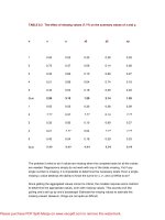
2.4 Scale Measurement Example




As an example demonstrating the different types of measurement scales, and the
measurements on those scales, almost anything might be chosen. I look around and see
my two dogs. These are things that appear as measurable objects in the real world and
will make a good example, as shown in Table 2.1.




TABLE 2.1 Title will go here







Scale Type

Measurement





Measured Value





Note








Nominal

Name





•

Fuzzy



•

Zeus





Distinguishes one from
the other.





Categorical

Breed





•

Golden
Retriever



•

Golden
Retriever





Could have chosen
other categories.

Categorical
(Dichotomous)




Gender





•

Female



•

Male

Categorical
(Binary)




Shots up to
Date
(1=Yes;0=No)





•

1



•

1

Please purchase PDF Split-Merge on www.verypdf.com to remove this watermark.


Categorical
(Missing)




Eye color





•

Value exists in
real world

Categorical
(Empty)




Drivers
License #





•

No such value
in real world










Ordinal

Fur length





•

Longer



•

Shorter





Comparative length
allowing ranking.

Interval




Date of Birth





•

1992



•

1991

Ratio




Weight





•

78 lbs



•

81 lbs

Ratio
(Dimensionless)




Height /
Length





•

0.5625



•

0.625


2.5 Transformations and Difficulties—Variables, Data, and
Information

Much of this discussion has pivoted on information—information in a data set, information
content of various scales, and transforming information. The concept of information is
crucial to data mining. It is the very substance enfolded within a data set for which the
data set is being mined. It is the reason to prepare the data set for mining—to best expose
the information contained in it to the mining tool. Indeed, the whole purpose for mining
data is to transform the information content of a data set that cannot be directly used and
understood by humans into a form that can be understood and used.




Part of Chapter 11 takes a more detailed look at some of the technical aspects of
information theory, and how they can be usefully used in the data preparation process.
Information theory provides very powerful and useful tools, not only for preparing data, but
also for understanding exactly what is enfolded in a data set. However, while within the
confines of information theory the term “information” has a mathematically precise
definition, Claude Shannon, principal pioneer of information theory, also provided a very
apt and succinct definition of the word. In the seminal 1949 work The Mathematical
Theory of Communication, Claude E. Shannon and Warren Weaver defined information
as “that which reduces uncertainty.” This is about as concise and practical a definition of
information as you can get.


Please purchase PDF Split-Merge on www.verypdf.com to remove this watermark.


Data forms the source material that the miner examines for information. The extracted
information allows better predictions of the behavior of some aspect of the world. The
improved prediction means, of necessity, that the level of uncertainty about the outcome is

reduced. Incorporating the information into a predictive or inferential framework provides
knowledge of how to act in order to bring about some desired result. The information will
usually not be perfect, so some uncertainty will remain, perhaps a great deal, and thus the
knowledge will not be complete. However, the better the information, the more predictive or
powerfully inferential the knowledge framework model will be.


2.6 Building Mineable Data Representations




In order to use the variables for mining, they have to be in the form of data. Originally the
word “datum” was used to indicate the same concept that is indicated here, in part, by
“measurement” or “value.” That is, a datum was a single instance value of a variable.
Here measurement both signifies a datum, and also is extended to indicate the values of
several features (variables) taken under some validating condition.




A collection of data points was called data, and the word was also used as a plural form of
datum. Computer users are more familiar with using data as a singular noun, which is the
style adopted here. However, there is more to the use of the term than simply a collection
of individual measurements. Data, at least as a source for mining, implies that the data
points, the values of the measurements, are all related in some identifiable way. One of
the ways the variables have to be structured has already been mentioned—they have to
have some validating phenomenon associated with a set of measurements. For example,
with each instance of a customer of cellular phone service who decides to leave a carrier,
a process called churning, the various attributes are captured and associated together.

The validating phenomenon for data is an intentional feature of the data, an integral part
of the way the data is structured. There are many other intentional features of data,
including basic choices such as what measurements to include and what degree of
precision to use for the measurements. All of the intentional, underlying assumptions and
choices form the superstructure for the data set. Three types of structure are discussed in
the next chapter. Superstructure, however, is the only one specifically involved in turning
variables into data.




Superstructure forms the framework on which the measurements hang. It is the
deliberately erected scaffolding that supports the measurements and turns them into data.
Putting such scaffolding in place and adding many instances of measured values is what
makes a data set. Superstructure plus instance values equals data sets.




2.6.1 Data Representation




The sort of data that is amenable to mining is always available on a computer system.

Please purchase PDF Split-Merge on www.verypdf.com to remove this watermark.
This makes discussions of data representation easy. Regardless of how the internal
operations of the computer system represent the data, whether a single computer or a
network, data can almost universally be accessed in the form of a table. In such a table
the columns represent the variables, and the records, or rows, represent instances. This
representation has become such a standardized form that it needs little discussion. It is
also very convenient that this standard form can also easily be discussed as a matrix, with
which the table is almost indistinguishable. Not only is the table indistinguishable from a
matrix for all practical purposes, but both are indistinguishable from a spreadsheet.



Spreadsheets are of limited value in actual mining due to their limited data capacity and
inability to handle certain types of operations needed in data preparation, data surveying,
and data modeling. For exploring small data sets, and for displaying various aspects of
what is happening, spreadsheets can be very valuable. Wherever such visualization is
used, the same row/column assumption is made as with a table.




So it is that throughout the book the underlying assumption about data representation is
that the data is present in a matrix, table, or spreadsheet format and that, for discussion
purposes, such representation is effectively identical and in every way equivalent.
However, it is not assumed that all of the operations described can be carried out in any of
the three environments. Explanations in the text of actual manipulations, and the
demonstration code, assume only the table structure form of data representation.

2.6.2 Building Data—Dealing with Variables




The data representation can usefully be looked at from two perspectives: as data and as a
data set. The terms “data” and “data set” are used to describe the different ways of
looking at the representation. Data, as used here, implies that the variables are to be
considered as individual entities, and their interactions or relationships to other variables
are secondary. When discussing the data set, the implication is that not only the variables
themselves are considered, but the interactions and interrelationships have equal or
greater import. Mining creates models and operates exclusively on data sets. Preparation
for mining involves looking at the variables individually as well as looking at the data set
as a whole.




Variables can be characterized in a number of useful ways as described in this chapter.
Having described some features of variables, we now turn our attention to the types of
actions taken to prepare variables and to some of the problems that need to be
addressed.




Variables as Objects

In order to find out if there are problems with the variables, it is necessary to look at a
summary description and discover what can be learned about the makeup of the variable
itself. This is the foundation and source material for deciding how to prepare each

Please purchase PDF Split-Merge on www.verypdf.com to remove this watermark.
variable, as well as where the miner looks at the variable itself as an object and
scrutinizes its key features and measurements.



Naturally it is important that the measurements about the variable are actually valid. That
is to say, any inferences made about the state of the features of the variable represent the
actual state of the variable. How could it be that looking at the variable wouldn’t reveal the
actual state of the variable? The problem here is that it may be impossible to look at all of
the instances of a variable that could exist. Even if it is not actually impossible, it may be
impractical to look at all of the instances available. Or perhaps there are not enough
instance values to represent the full behavior of the variable. This is a very important
topic, and Chapter 5 is entirely dedicated to describing how it is possible to discover if
there is enough data available to come to valid conclusions. Suffice it to say, it is
important to have enough representative data from which to draw any conclusions about
what needs to be done.




Given that enough data is available, a number of features of the variable are inspected.
Whatever it is that the features discover, each one inspected yields insight into the
variable’s behavior and might indicate some corrective or remedial action.

Removing Variables




One of the features measured is a count of the number of instance values. In any sample
of values there can be only a limited number of different values, that being the size of the
sample. So a sample of 1000 can have at most only 1000 distinct values. It may very well
be that some of the values occur more than once in the sample. In some cases—1000
binary variable instances, for example—it is certain that multiple occurrences exist.




The basic information comprises the number of distinct values and the frequency count of
each distinct value. From this information it is easy to determine if a variable is entirely
empty—that is, that it has only a single value, that of “empty” or “missing.” If so, the
variable can be removed from the data set. Similarly, constants are discovered and can
also be discarded.




Variables with entirely missing values and variables that contain only a single value can
be discarded because the lack of variation in content carries no information for modeling
purposes. Information is only carried in the pattern of change of value of a variable with

changing circumstances. No change, no information.




Removing variables becomes more problematic when most of the instance values are
empty, but occasionally a value is recorded. The changing value does indeed present
some information, but if there are not many actual values, the information density of the
variable is low. This circumstance is described as sparsity.




Sparsity


Please purchase PDF Split-Merge on www.verypdf.com to remove this watermark.


When individual variables are sparsely populated with instance values, the miner needs to
decide when to remove them because they have insignificant value. Chapter 5 describes
in some detail how to decide when to remove sparse variables. Essentially, the miner has
to make an arbitrary decision about confidence levels, that is, how confident the miner
needs to be in the model.




There is more to consider about sparsity, however, than can be seen by considering
variables individually. In some modeling applications, sparsity is a very large problem. In

several applications, such as in telecommunications and insurance, data is collected in
ways that generate very sparsely populated data sets. The variable count can be high in
some cases, over 7000 variables in one particular case, but with many of the variables
very sparsely populated indeed. In such a case, the sparsely populated variables are not
removed. In general, mining tools deal very poorly with highly sparse data. In order to be
able to mine them, they need to be collapsed into a reduced number of variables in such a
way that each carries information from many of the original variables. Chapter 10
discusses collapsing highly sparse data.




Since each of the instances are treated as points in state space, and state space has
many dimensions, reducing the number of variables is called dimensionality reduction, or
collapsing dimensionality. Techniques for dealing with less extreme sparsity, but when
dimensionality reduction is still needed, are discussed in Chapter 7. State space is
described in more detail in Chapter 6.




Note that it has to be the miner’s decision if a particular variable should be eliminated
when some sparsity threshold is reached, or if the variable should be collapsed in
dimensionality with other variables. The demonstration software makes provision for
flagging variables that need to be retained and collapsed. If not flagged, the variables are
treated individually and removed if they fall below the selected sparsity threshold.

Monotonicity




A monotonic variable is one that increases without bound. Monotonicity can also exist in
the relationship between variables in which as one variable increases, the other does not
decrease but remains constant, or also increases. At the moment, while discussing
variable preparation, it is the monotonic variable itself that is being considered, not a
monotonic relationship.




Monotonic variables are very common. Any variable that is linked to the passage of time,
such as date, is a monotonic variable. The date always increases. Other variables not
directly related to time are also monotonic. Social security numbers, record numbers,
invoice numbers, employee numbers, and many, many other such indicators are
monotonic. The range of such categorical or nominal values increases without bound.



Please purchase PDF Split-Merge on www.verypdf.com to remove this watermark.

The problem here is that they almost always have to be transformed into some
nonmonotonic form if they are to be used in mining. Unless it is certain that every possible
value of the monotonic variable that will be used is included in the data set, transformation
is required. Transformation is needed because only some limited part of the full range of
values can possibly be included in any data set. Any other data set, specifically the
execution data set, will contain values of the monotonic variable that were not in the

training data set. Any model will have no reference for predicting, or inferring, the meaning
of the values outside its training range. Since the mined model will not have been
exposed to such values, predictions or inferences based on such a model will at best be
suspect.




There are a number of transformations that can be made to monotonic variables,
depending on their nature. Datestamps, for instance, are often turned into seasonality
information in which the seasons follow each other consecutively. Another transformation
is to treat the information as a time series. Time series are treated in several ways that
limit the nature of the monotonicity, say, by comparing “now” to some fixed distance of
time in the past. Unfortunately, each type of monotonic variable requires specific
transformations tailored to best glean information from it. Employee numbers will no doubt
need to be treated differently from airline passenger ticket numbers, and those again from
insurance policy numbers, and again from vehicle registration numbers. Each of these is
monotonic and requires modification if they are to be of value in mining.




It is very hard to detect a monotonic variable in a sample of data, but certain detectable
characteristics point to the possibility that a variable is in fact monotonic. Two measures
that have proved useful in giving some indication of monotonicity in a variable (described
in Chapter 5) are interstitial linearity and rate of detection. Interstitial linearity measures
the uniformity of spacing between the sampled values, which tends to be more uniform in
a monotonic variable than in some nonmonotonic ones. Rate of discovery measures the
rate at which new values are experienced during random sampling of the data set. Rate of
detection tends to remain uniform for monotonic variables during the whole sampling

period and falls off for some nonmonotonic variables.




A problem with these metrics is that there are nonmonotonic variables that also share the
characteristics that are used to detect potential monotonicity. Nonetheless, used as
warning flags that the variables indicated need looking at more closely for monotonicity or
other problems, the metrics are very useful. As noted, automatically modifying the
variables into some different form is not possible.




Increasing Dimensionality




The usual problem in mining large data sets is in reducing the dimensionality. There are
some circumstances where the dimensionality of a variable needs to be increased. One
concern is to increase the dimensionality as much as is needed, but only as little as
necessary, by recoding and remapping variables. Chapter 7 deals in part with these

Please purchase PDF Split-Merge on www.verypdf.com to remove this watermark.
techniques. The types of variables requiring this transformation, which are almost always
categorical, carry information that is best exposed in more than one dimension. A couple
of examples illustrate the point.

Colors can be represented in a variety of ways. Certainly a categorical listing covers the
range of humanly appreciated color through a multitude of shades. Equally well, for some
purposes, the spectral frequency might be listed. However, color has been usefully
mapped onto a color wheel. Such a wheel not only carries color information, but also
describes color as a continuum, carrying information about what other colors are near and
far from some selected category. This is very useful information. Since a circle can be
drawn on a plane, such as a piece of paper, it is easy to see that any point on the circle’s
circumference can be unambiguously represented by two coordinates, or numbers.
Mapping the color wheel onto a circle on a graph and using the two coordinates for some
selected color as the instance values of two variables may form a better description of
color than a categorical listing.




ZIP codes form a perennial problem in mining. Sometimes, depending on the application,
it is beneficial to translate the ZIP code from the categorical list into latitude and longitude.
These values translate the ZIP code into two instance values. The single variable “ZIP”
translates into two variables, say, “Lat” and “Lon.”




Once again, the decision of whether to expand the dimensionality of a variable must be, in
many cases, left up to the miner or domain expert.

Outliers




An outlier is a single, or very low frequency, occurrence of the value of a variable that is
far away from the bulk of the values of the variable. The question miners always ask is: “Is
this a mistake?” As a general rule of thumb, if it can be established that it is a mistake, it
can be rectified. (One way to do this, if the correct value cannot be found, is to treat it as a
missing value, discussed later in this chapter.) The problem is what to do if it cannot be
pinpointed as an error. It is a problem because, for some modeling methods in particular
(some types of neural network, for instance), outliers may distort the remaining data to the
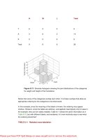
point of uselessness. Figure 2.5(a) shows this sort of situation.



Please purchase PDF Split-Merge on www.verypdf.com to remove this watermark.






Figure 2.5 Examples of outliers: as an individual value (a) and as clumps of
values (b).

Insurance data typically suffers considerably from the problem of outliers. Most insurance
claims are small, but occasionally one comes in for some enormous sum. This is no error,
and it must be included in modeling. How to do this without distorting the remaining data is
a problem.




There is also a problem when the outliers are not individual values but clumps of values,
illustrated in Figure 2.5(b). It’s actually the gaps between the clumps that can pose
problems. Are these clumps, perhaps, valid measurements from differently biased
instruments? Once again, it must be determined first that there is not some sort of error.
Maybe some measurements were made against an incorrect calibration and are biased.
However, again it might not be possible to determine that an error occurred. In general,
the miner is constrained to consider that the measurements are not an error until and
unless it is possible to definitely show that they are.




If indeed the outlying value is not a mistake, or is at least going to be dealt with as if it is
not, how is it to be treated? Fortunately there is a way of automatically dealing with the
problem if it is not a mistake. This involves remapping the variable’s values. Part of
Chapter 7 deals with this remapping.




Numerating Categorical Values

Dealing correctly with categorical values is one of the most important functions of data
preparation. For many modeling techniques it is necessary to translate categorical values
into numbers: they simply cannot deal with untranslated categorical values. Experience
shows that even modeling techniques that can deal well with untranslated categorical
values benefit from a valid numeration of categoricals.




However, a na‹ve way of making the translation, one that is very commonly done, is
terribly destructive of information. Simply assigning numbers to the nominals to create a

Please purchase PDF Split-Merge on www.verypdf.com to remove this watermark.