Data Preparation for Data Mining- P6

(49 + 63 + 44 + 25 + 16)/5 = 39.4




so squaring the instance value minus the mean:




(49 – 39.4)
2
= 9.6
2
= 92.16
(63 – 39.4)
2
= 23.6
2
= 556.96
(44 – 39.4)
2
= 4.6
2
= 21.16
(25 – 39.4)
2
= –14.4
2

= 207.36
(16 – 39.4)
2
= –23.4
2
= 547.56




and since the variance is the mean of these differences:




(92.16 + 556.96 + 21.16 + 207.36 + 547.56)/5 = 285.04




This number, 285.04, is the mean of the squares of the differences. It is therefore a
variance of 285.04 square units. If these numbers represent some item of interest, say,
percentage return on investments, it turns out to be hard to know exactly what a variance
of 285.04 square percent actually means. Square percentage is not a very familiar or
meaningful measure in general. In order to make the measure more meaningful in
everyday terms, it is usual to take the square root, the opposite of squaring, which would
give 16.88. For this example, this would now represent a much more meaningful variance
of 16.88 percent.

The square root of the variance is called the standard deviation. The standard deviation is
a very useful thing to know. There is a neat, mathematical notation for doing all of the
things just illustrated:




Standard deviation =




where









means to take the square root of everything under it

Σ




means to sum everything in the brackets following it





x




is the instance value





m




is the mean

n




is the number of instances





(For various technical reasons that we don’t need to get into here, when the number is
divided by n, it is known as the standard deviation of the population, and when divided by

Please purchase PDF Split-Merge on www.verypdf.com to remove this watermark.
n – 1, as the standard deviation of the sample. For large numbers of instances, which will
usually be dealt with in data mining, the difference is miniscule.)



There is another formula for finding the value of the standard deviation that can be found
in any elementary work on statistics. It is the mathematical equivalent of the formula
shown above, but gives a different perspective and reveals something else that is going
on inside this formula—something that is very important a little later in the data
preparation process:

What appears in this formula is “Σx
2
,” which is the sum of the instance values squared.
Notice also that “nm
2
,” which is the number of instances multiplied by the mean, squared.
Since the mean is just the sum of the x values divided by the number of values (or Σx/n),
the formula could be rewritten as









But notice that n(Σx/n) is the same as Σx, so the formula becomes

(being careful to note that Σx
2
means to add all the values of x squared, whereas (Σx)
2

means to take the sum of the unsquared x values and square the total).




This formula means that the standard deviation can be determined from three separate
pieces of information:




1.

The sum of x
2
, that is, adding up all squares of the instance values




2.

The sum of x, that is, adding up all of the instance values




3.

The number of instances




The standard deviation can be regarded as exploring the relationship among the sum of
the squares of the instance values, the sum of the instance values, and the number of
instances. The important point here is that in a sample that contains a variety of different
values, the exact ratio of the sum of the numbers to the sum of the squares of the
numbers is very sensitive to the exact proportion of numbers of different sizes in the
sample. This sensitivity is reflected in the variance as measured by the standard
deviation.



Please purchase PDF Split-Merge on www.verypdf.com to remove this watermark.

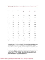
Figure 5.5 shows distribution curves for three separate samples, each from a different
population. The range for each sample is 0–100. The linear (or rectangular) distribution
sample is a random sample drawn from a population in which each number 0–100 has an
equal chance of appearing. This sample is evidently not large enough to capture this
distribution well! The bimodal sample was drawn from a population with two “humps” that

do show up in this limited sample. The normal sample was drawn from a population with a
normal distribution—one that would resemble the “bell curve” if a large enough sample
was taken. The mean and standard deviation for each of these samples is shown in Table
5.1.









Figure 5.5 Distribution curves for samples drawn from three populations.






TABLE 5.1 Sample statistics for three distributions.







Sample
distribution

Mean





Standard
deviation








Linear




47.96

29.03





Bimodal




49.16





17.52





Normal




52.39

11.82








The standard deviation figures indicate that the linear distribution has the highest
variance, which is not surprising as it would be expected to have the greatest average
distance between the sample mean and the instance values. The normal distribution

Please purchase PDF Split-Merge on www.verypdf.com to remove this watermark.
sample is the most bunched together around its sample mean and has the least standard
deviation. The bimodal is more bunched than the linear, and less than the normal, and its
standard deviation indicates this, as expected.



Standard deviation is a way to determine the variability of a sample that only needs to have
the instance values of the sample. It results in a number that represents how the instance
values are scattered about the average value of the sample.

5.2 Confidence




Now that we have an unambiguous way of measuring variability, actually capturing it
requires enough instances of the variable so that the variability in the sample matches the
variability in the population. Doing so captures all of the structure in the variable.
However, it is only possible to be absolutely 100% certain that all of the variability in a
variable has been captured if all of the population is included in the sample! But as we’ve
already discussed, that is at best undesirable, and at worst impossible. Conundrum.




Since sampling the whole population may be impossible, and in any case cannot be
achieved when it is required to split a collected data set into separate pieces, the miner
needs an alternative. That alternative is to establish some acceptable degree of
confidence that the variability of a variable is captured.




For instance, it is common for statisticians to use 95% as a satisfactory level of
confidence. There is certainly nothing magical about that number. A 95% confidence
means, for instance, that a judgment will be wrong 1 time in 20. That is because, since it is
right 95 times in 100, it must be wrong 5 times in 100. And 5 times in 100 turns out to be 1
time in 20. The 95% confidence interval is widely used only because it is found to be
generally useful in practice. “Useful in practice” is one of the most important metrics in
both statistical analysis and data mining.

It is this concept of “level of confidence” that allows sampling of data sets to be made. If
the miner decided to use only a 100% confidence level, it is clear that the only way that
this can be done is to use the whole data set complete as a sample. A 100% sample is
hardly a sample in the normal use of the word. However, there is a remarkable reduction
in the amount of data needed if only a 99.99% confidence is selected, and more again for
a 95% confidence.




A level of confidence in this context means that, for instance, it is 95% certain that the
variability of a particular variable has been captured. Or, again, 1 time in 20 the full variability
of the variable would not have been captured at the 95% confidence level, but some lesser
level of variability instead. The exact level of confidence may not be important. Capturing
enough of the variability is vital.


5.3 Variability of Numeric Variables


Please purchase PDF Split-Merge on www.verypdf.com to remove this watermark.


Variability of numeric variables is measured differently from the variability of nonnumeric
variables. When writing computer code, or describing algorithms, it is easy to abbreviate
numeric and nonnumeric to the point of confusion—“Num” and “Non.” To make the

difference easier to describe, it is preferable to use distinctive abbreviations. This
distinction is easy when using “Alpha” for nominals or categoricals, which are measured in
nonnumeric scales, and “Numeric” for variables measured using numeric scales. Where
convenient to avoid confusion, that nomenclature is used here.




Variability of numeric variables has been well described in statistical literature, and the
previous sections discussing variability and the standard deviation provide a conceptual
overview.




Confidence in variability capture increases with sample size. Recall that as a sample size
gets larger, so the sample distribution curve converges with the population distribution
curve. They may never actually be identical until the sample includes the whole
population, but the sample size can, in principle, be increased until the two curves
become as similar as desired. If we knew the shape of the population distribution curve, it
would be easy to compare the sample distribution curve to it to tell how well the sample
had captured the variability. Unfortunately, that is almost always impossible. However, it is
possible to measure the rate of change of a sample distribution curve as instance values
are added to the sample. When it changes very little with each addition, we can be
confident that it is closer to the final shape than when it changes faster. But how
confident? How can this rate of change be turned into a measure of confidence that
variability has been captured?

5.3.1 Variability and Sampling




But wait! There is a critical assumption here. The assumption is that a larger sample is in
fact more representative of the population as a whole than a smaller one. This is not
necessarily the case. In the forestry example, if only the oldest trees were chosen, or only
those in North America, for instance, taking a larger sample would not be representative.
There are several ways to assure that the sample is representative, but the only one that
can be assured not to introduce some bias is random sampling. A random sample
requires that any instance of the population is just as likely to be a member of the sample
as any other member of the population. With this assumption in place, larger samples will,
on average, better represent the variability of the population.




It is important to note here that there are various biases that can be inadvertently
introduced into a sample drawn from a population against which random sampling
provides no protection whatsoever. Various aspects of sampling bias are discussed in
Chapters 4 and 10. However, what a data miner starts with as a source data set is almost
always a sample and not the population. When preparing variables, we cannot be sure
that the original data is bias free. Fortunately, at this stage, there is no need to be. (By

Please purchase PDF Split-Merge on www.verypdf.com to remove this watermark.
Chapter 10 this is a major concern, but not here.) What is of concern is that the sample
taken to evaluate variable variability is representative of the original data sample. Random
sampling does that. If the original data set represents a biased sample, that is evaluated

partly in the data assay (Chapter 4), again when the data set itself is prepared (Chapter
10), and again during the data survey (Chapter 11). All that is of concern here is that, on a
variable-by-variable basis, the variability present in the source data set is, to some
selected level of confidence, present in the sample extracted for preparation.



5.3.2 Variability and Convergence




Differently sized, randomly selected samples from the same population will have different
variability measures. As a larger and larger random sample is taken, the variability of the
sample tends to fluctuate less and less between the smaller and larger samples. This
reduction in the amount of fluctuation between successive samples as sample size
increases makes the number measuring variability converge toward a particular value.




It is this property of convergence that allows the miner to determine a degree of
confidence about the level of variability of a particular variable. As the sample size
increases, the average amount of variability difference for each additional instance
becomes less and less. Eventually the miner can know, with any arbitrary degree of
certainty, that more instances of data will not change the variability by more than a
particular amount.

Figure 5.6 shows what happens to the standard deviation, measured up the side of the
graph, as the number of instances in the sample increases, which is measured along the
bottom of the graph. The numbers used to create this graph are from a data set provided
on the CD-ROM called CREDIT. This data set contains a variable DAS that is used
through the rest of the chapter to explore variability capture.









Figure 5.6 Measuring variability DAS in the CREDIT data set. Each sample
contains one more instance than the previous sample. As the sample size
increases, the variability seems to approach, or converge, toward about 130.

Please purchase PDF Split-Merge on www.verypdf.com to remove this watermark.





Figure 5.6 shows incremental samples, starting with a sample size of 0, and increasing
the sample size by one each time. The graph shows the variability in the first 100
samples. Simply by looking at the graph, intuition suggests that the variability will end up
somewhere about 130, no matter how many more instances are considered. Another way
of saying this is that it has converged at about 130. It may be that intuition suggests this to

be the case. The problem now is to quantify and justify exactly how confident it is possible
to be. There are two things about which to express a level of confidence—first, to specify
exactly the expected limits of variability, and second, to specify how confident is it
possible to be that the variability actually will stay within the limits.




The essence of capturing variability is to continue to add samples until both of those
confidence measures can be made at the required level—whatever that level may be.
However, before considering the problem of justifying and quantifying confidence, the next
step is to examine capturing variability in alpha-type variables.


5.4 Variability and Confidence in Alpha Variables




So far, much of this discussion has described variability as measured in numeric
variables. Data mining often involves dealing with variables measured in nonnumeric
ways. Sometimes the symbolic representation of the variable may be numeric, but the
variable still is being measured nominally—such as SIC and ZIP codes.




Measuring variability in these alpha-type variables is every bit as important as in
numerical variables. (Recall this is not a new variable type, just a clearer name for
qualitative variables—nominals and categoricals—to save confusion.)

A measure of variability in alpha variables needs to work similarly to that for numeric
variables. That is to say, increases in sample size must lead to convergence of variability.
This convergence is similar in nature to that of numerical variables. So using such a
method, together with standard deviation for numeric variables, gives measures of
variability that can be used to sample both alpha and numeric variables. How does such a
method work?




Clearly there are some alpha variables that have an almost infinite number of
categories—people’s names, for instance. Each name is an alpha variable (a nominal in
the terminology used in Chapter 2), and there are a great many people each with different
names!




For the sake of simplicity of explanation, assume that only a limited number of alpha
labels exist in a variable scale. Then the explanation will be expanded to cover alpha
variables with very high numbers of distinct values.



Please purchase PDF Split-Merge on www.verypdf.com to remove this watermark.

In a particular population of alpha variables there will be a specific number of instances of
each of the values. It is possible in principle to count the number of instances of each
value of the variable and determine what percentage of the time each value occurs. This
is exactly similar to counting how often each numeric instance value occurred when
creating the histogram in Figure 5.1. Thus if, in some particular sample, “A” occurred 124
times, “B” 62 times, and “C” 99 times, then the ratio of occurrence, one to the others, is as
shown in Table 5.2.




TABLE 5.2 Sample value frequency counts.







Sample
distribution




Mean

Standard
deviation








A




124





43.51





B

62





21.75





C




99





34.74

Total




285





100.00








If the population is sampled randomly, this proportion will not be immediately apparent.
However, as the sample size increases, the relative proportion will become more and
more nearly what is present in the population; that is, it converges to match that of the
population. This is altogether similar to the way that the numeric variable variability
converges. The main difference here is that since the values are alpha, not numeric,
standard deviation can’t be calculated.

Instead of determining variability using standard deviation, which measures the way
numeric values are distributed about the mean, alpha variability measures the rate of
change of the relative proportion of the values discovered. This rate of change is
analogous to the rate of change in variability for numerics. Establishing a selected degree
of confidence that the relative proportion of alpha values will not change, within certain
limits, is analogous to capturing variability for a numeric variable.




5.4.1 Ordering and Rate of Discovery




One solution to capturing the variability of alpha variables might be to assign numbers to

Please purchase PDF Split-Merge on www.verypdf.com to remove this watermark.
each alpha and use those arbitrarily assigned numbers in the usual standard deviation
formula. There are several problems with this approach. For one thing, it assumes that
each alpha value is equidistant from one another. For another, it arbitrarily assigns an
ordering to the alphas, which may or may not be significant in the variability calculation,
but certainly doesn’t exist in the real world for alphas other than ordinals. There are other
problems so far as variability capture goes also, but the main one for sampling is that it
gives no clue whether all of the unique alpha values have been seen, nor what chance
there is of finding a new one if sampling continues. What is needed is some method that
avoids these particular problems.

Numeric variables all have a fixed ordering. They also have fixed distances between
values. (The number “1” is a fixed distance from “10”—9 units.) These fixed relationships
allow a determination of the range of values in any numeric distribution (described further
in Chapter 7). So for numeric variables, it is a fairly easy matter to determine the chance
that new values will turn up in further sampling that are outside of the range so far
sampled.




Alphas have no such fixed relationship to one another, nor is there any order for the alpha
values (at this stage). So what is the assurance that the variability of an alpha variable has
been captured, unless we know how likely it is that some so far unencountered value will
turn up in further sampling? And therein lies the answer—measuring the rate of discovery
of new alpha values.




As the sample size increases, so the rate of discovery (ROD) of new values falls. At first,
when the sample size is low, new values are often discovered. As the sampling goes on,
the rate of discovery falls, converging toward 0. In any fixed population of alphas, no
matter how large, the more values seen, the less new ones there are to see. The chance
of seeing a new value is exactly proportional to the number of unencountered values in
the population.

For some alphas, such as binary variables, ROD falls quickly toward 0, and it is soon easy to
be confident (to any needed level of confidence) that new values are very unlikely. With
other alphas—such as, say, a comprehensive list of cities in the U.S.—the probability would
fall more slowly. However, in sampling alphas, because ROD changes, the miner can
estimate to any required degree of confidence the chance that new alpha values will turn up.
This in turn allows an estimate not only of the variability of an alpha, but of the
comprehensiveness of the sample in terms of discovering all the alpha labels.


5.5 Measuring Confidence




Measuring confidence is a critical part of sampling data. The actual level of confidence
selected is quite arbitrary. It is selected by the miner or domain expert to represent some
level of confidence in the results that is appropriate. But whatever level is chosen, it is so
important in sampling that it demands closer inspection as to what it means in practice,

Please purchase PDF Split-Merge on www.verypdf.com to remove this watermark.
and why it has to be selected arbitrarily.



5.5.1 Modeling and Confidence with the Whole Population

If the whole population of instances were available, predictive modeling would be quite
unnecessary. So would sampling. If the population really is available, all that needs to be
done to “predict” the value of some variable, given the values of others, is to look up the
appropriate case in the population. If the population is truly present, it is possible to find an
instance of measurements that represents the exact instance being predicted—not just
one similar or close to it.




Inferential modeling would still be of use to discover what was in the data. It might provide
a useful model of a very large data set and give useful insights into related structures. No
training and test sets would be needed, however, because, since the population is
completely represented, it would not be possible to overtrain. Overtraining occurs when
the model learns idiosyncrasies present in the training set but not in the whole population.
Given that the whole population is present for training, anything that is learned is, by
definition, present in the population. (An example of this is shown in Chapter 11.)




With the whole population present, sampling becomes a much easier task. If the
population were too large to model, a sample would be useful for training. A sample of
some particular proportion of the population, taken at random, has statistically well known
properties. If it is known that some event happens in, say, a 10% random sample with a
particular frequency, it is quite easy to determine what level of confidence this implies
about the frequency of the event in the population. When the population is not available,
and even the size of the population is quite unknown, no such estimates can be made.
This is almost always the case in modeling.

Because the population is not available, it is impossible to give any level of confidence in
any result, based on the data itself. All levels of confidence are based on assumptions
about the data and about the population. All kinds of assumptions are made about the
randomness of the sample and the nature of the data. It is then possible to say that if
these assumptions hold true, then certain results follow. The only way to test the
assumptions, however, is to look at the population, which is the very thing that can’t be
done!




5.5.2 Testing for Confidence




There is another way to justify particular levels of confidence in results. It relies on the
quantitative discriminatory power of tests. If, for instance, book reviewers can consistently
and accurately predict a top 10 best-selling book 10% of the time, clearly they are wrong
90% of the time. If a particular reviewer stated that a particular book just reviewed was
certain to be a best-seller, you would be justified in being skeptical of the claim. In fact,
you would be quite justified in being 10% sure (or confident) that it would be a success,

Please purchase PDF Split-Merge on www.verypdf.com to remove this watermark.
and 90% confident in its failure. However, if at a convention of book reviewers, every one
of hundreds or thousands of reviewers each separately stated that the book was sure to
be a best-seller, even though each reviewer had only a 10% chance of success, you

would become more and more convinced of the book’s chance of success.



Each reviewer performs an independent reading, or test, of the book. It is this
independence of tests that allows an accumulation of confidence. The question is, how
much additional confidence is justified if two independent tests are made, each with a
10% accuracy of being correct in their result, and both agree? In other words, suppose
that after the first reviewer assured you of the book’s success, a second one did the
same. How much more confident, if at all, are you justified in being as a result of the
second opinion? What happens if there are third and fourth confirming opinions? How
much additional confidence are you justified in feeling?




At the beginning you are 100% skeptical. The first reviewer’s judgment persuades you to
an opinion of 10% in favor, 90% against the proposition for top 10 success. If the first
reviewer justified a 10/90% split, surely the second does too, but how does this change
the level of confidence you are justified in feeling?




Table 5.3 shows that after the first reviewer’s assessment, you assigned 10% confidence
to success and 90% to skepticism. The second opinion (test) should also justify the
assignment of an additional 10%. However, you are now only 90% skeptical, so it is 10%
of that 90% that needs to be transferred, which amounts to an additional 9% confidence.
Two independent opinions justify a 19% confidence that the book will be a best-seller.
Similar reasoning applies to opinions 3, 4, 5, and 6. More and more positive opinions

further reinforce your justified confidence of success. With an indefinite amount of
opinions (tests) available, you can continue to get opinions until any particular level of
confidence in success is justified.




TABLE 5.3 Reviewer assurance charges confidence level.







Reviewer
number




Start
level





Transfer
amount

(start
level x10%)





Confidence
of success





Your remaining
skeptical balance








1




100%

10





10





90





2




90%

9





9





81











Please purchase PDF Split-Merge on www.verypdf.com to remove this watermark.

3



81%



8.1



27.1



72.9




4




72.9%

7.29





34.39





65.61





5




65.61%

6.561





40.951





59.049





6




59.049%

5.9049%





46.8559





53.1441








Of course, a negative opinion would increase your skepticism and decrease your
confidence in success. Unfortunately, without more information it is impossible to say by
how much you are justified in revising your opinion. Why?




Suppose each reviewer reads all available books and predicts the fate of all of them. One
month 100 books are available, 10 are (by definition) on the top 10 list. The reviewer

predicts 10 as best-sellers and 90 as non-best-sellers. Being consistently 10% accurate,
one of those predicted to be on the best-seller list was on it, 9 were not. Table 5.4 shows
the reviewer’s hit rate this month.




TABLE 5.4 Results of the book reviewer’s predictions for month 1.







Month 1




Best-seller





Non-best seller

Predicted bestseller




1





9





Predicted non-best-seller




9

81








Since one of the 10 best-sellers was predicted correctly, we see a 10% rate of accuracy.
There were also 90 predicted to be non-best-sellers, of which 81 were predicted correctly
as non-best-sellers. (81 out of 90 = 81/90 = 90% incorrectly predicted.)




In month 2 there were 200 books published. The reviewer read them all and made 10
best-seller predictions. Once again, a 10% correct prediction was achieved, as Table 5.5
shows.




TABLE 5.5 Results of the book reviewer’s predictions for month 2.

Please purchase PDF Split-Merge on www.verypdf.com to remove this watermark.