Điện tử viễn thông lect10 1 khotailieu
Bạn đang xem bản rút gọn của tài liệu. Xem và tải ngay bản đầy đủ của tài liệu tại đây (642.78 KB, 36 trang )
10. Network models
lect10.ppt
S-38.1145 – Introduction to Teletraffic Theory – Spring 2006
1
10. Network models
Contents
•
•
Circuit switched network modelled as a loss network
Packet switched network modelled as a queueing network
2
10. Network models
Teletraffic model of a circuit switched network (1)
•
Consider a circuit switched
network
B
– e.g. a telephone network
•
Traffic:
– telephone calls
– each (carried) call occupies one
channel on each link among its
route
•
A
System:
– telephone machines (terminals)
– exchanges (network nodes)
– access links (from terminals to
exchanges)
– trunks (between exchanges)
3
10. Network models
Teletraffic model of a circuit switched network (2)
•
Quality of service:
B
– described by the end-to-end
call blocking probability
(prob. that a desired connection
cannot be set up due to
congestion along the route of
the connection)
•
In our model we assume that
A
– the network nodes and the
whole access network are nonblocking
•
Thus, a call is blocked
– if and only if all channels are
occupied in any trunk network
link along the route of that call
4
10. Network models
Links j = 1,…,J
•
In our model,
B
– all links are two-way (why?)
•
•
•
We index the links in the trunk
network by
– j = 1,…,J
– example on the right: J = 6
Let nj denote the number of
channels in link j (that is: the link
capacity)
– n = (n1,…,nJ)
Each link is modelled as a
2
3
1
6
A
5
4
– pure loss system
5
10. Network models
Routes r = 1,…,R
•
We define a route as a
B
– set of consecutive (two-way)
links connecting two network
nodes
•
•
We index the routes by
– r = 1,…,R
In the example on the right:
– R = 12 + 10 + 7 + 3 = 32
– there are three routes
between nodes a and b:
{1,2}, {6,3}, {5,4,3}
•
2
b
3
1
A
6
a
5
4
Let djr = 1 if link j belongs to
route r (otherwise djr = 0)
– D = (djr | j = 1,…,J; r = 1,…,R)
6
10. Network models
Traffic classes
•
Note:
B
– End-to-end call blocking prob. is
equal for all the connections
following the same route
•
Thus the traffic class of a
connection is determined by the
route r the connection follows
– Example on the right: connection
between A and B belongs to
class using route {6,3}
•
•
2
b
3
1
A
6
a
5
4
Let xr denote the number of
active connections following
route r
– x = (x1,…,xR)
Vector x is called the state of the
system
7
10. Network models
State space
•
The number of active connections xr for any traffic class r is limited by
the link capacities nj along the corresponding route r :
R
∑ d jr xr ≤ n j for all j
r =1
•
The same in vector form:
D⋅ x≤n
•
Thus, the state space S (that is: the set of admissible states) is
S = {x ≥ 0 | D ⋅ x ≤ n}
– Note that, due to finite link capacities, set S is finite
8
10. Network models
Example
•
3 links with capacities:
– link a-c: 3 channels
– link b-c: 3 channels
– link c-d: 4 channels
•
2 routes:
3
c
4
d
b
4
– route a-c-d
– route b-c-d
– The other 4 routes (which?) are
ignored in this model
•
3
a
State space:
– S = {(0,0),(0,1),(0,2),(0,3),
(1,0),(1,1),(1,2),(1,3),
(2,0),(2,1),(2,2),
(3,0),(3,1)}
3
S
x2 2
1
0
0 1 2 3 4
x1
x1 ≥ 0
x2 ≥ 0
9
10. Network models
Set Sr of non-blocking states for class r
•
Consider
– an arriving call belonging to class r (that is: following route r)
•
It will not be blocked by link j belonging to route r
– if there is at least one free channel on link j:
R
∑ d jr ' xr ' ≤ n j − 1 for all j ∈ r
r '=1
•
The same in vector form (er being here the unit vector in direction r):
D ⋅ (x + e r ) ≤ n
•
The set Sr of non-blocking states for class r is thus
S r = {x ≥ 0 | D ⋅ (x + e r ) ≤ n}
10
10. Network models
Set SrB of blocking states for class r
•
The set SrB of blocking states
for class r is clearly:
S rB
•
= S \ Sr
c
d
b
Summary:
– an arriving call of class r is
blocked (and lost)
if and only if the state x of the
system belongs to set SrB
•
a
Example (continued):
– The blocking states S1B for
connections of class 1
(using route a-c-d) are
circulated in the figure
–
S1B = { (1,3),(2,2),(3,0),(3,1)}
4
3
x2 2
1
0
0 1 2 3 4
x1
11
10. Network models
Loss network
•
Assume that
– new connection requests belonging to traffic class r arrive (independently)
according to a Poisson process with intensity λr
– call holding times independently and identically distributed with mean h
•
Denote
– ar = λrh (traffic intensity for class r)
12
10. Network models
Equilibrium distribution (1)
•
Then it is possible to show that
– the stationary state probability π(x) for any state x ∈ S is as follows:
π (x ) = G
−1
R
⋅ ∏ f r ( xr )
r =1
where G is a normalizing constant:
R
G = ∑ ∏ f r ( xr )
x∈S r =1
and the functions fr(xr) are defined as follows:
a r xr
f r ( xr ) =
xr !
13
10. Network models
Equilibrium distribution (2)
•
Probability π(x) is said to be of product-form
– However, the number of active connections of different classes are not
independent (since the normalizing constant G depends on each xr)
– Only if all the links had infinite capacities,
all the traffic classes would be independent of each other
– Thus, it is the limited resources shared by the traffic classes
that makes them dependent on each other
14
10. Network models
PASTA
•
Consider, for a while,
– any simple teletraffic model with Poisson arrivals
•
According to so called PASTA (Poisson Arrivals See Time Averages)
property,
– arriving calls (obeying a Poisson process) see the system in equilibrium
•
This is an important observation
– applicable in many problems
•
For example,
– it allows us to calculate the end-to-end blocking probabilities in our circuit
switched network model (since we assumed that new calls arrive according
to a Poisson process)
15
10. Network models
End-to-end blocking: exact formula
•
The probability that the system is in a state such that it cannot accept
any more connections of type r is clearly given by the sum
∑ π ( x)
x∈ S rB
– Call this the end-to-end time blocking probability for class r
•
Due to the PASTA property,
– the end-to-end call blocking probability Br equals this:
Br = ∑ π ( x)
x∈ S rB
•
Since there is no difference between time and call blocking in this case,
we may briefly call it end-to-end blocking.
16
10. Network models
Example
•
Consider the example presented in slide 9 (and continued in slide 11)
•
The end-to-end blocking probability B1 for class 1 will be
B1 = π (1,3) + π ( 2 , 2 ) + π (3,0 ) + π (3,1) =
a11 a 23
1!3!
a12 a 22
2!2!
a13
3!
a12
+
+ 1 + 1!
a 12 a 22 a 23 a11
a12 a 22 a 23 a12
a12 a 22 a13
a12
1 +
+ 2! + 3! + 1! 1 + 1! + 2! + 3! + 2! 1 + 1! + 2! + 3! 1 + 1!
1!
17
10. Network models
Approximative methods
•
In practice,
– it is extremely hard (even impossible) to apply the exact formula
– This is due to the so called state space explosion:
there are as many dimensions in the state spaces as
there are routes in our model
⇒ exponential growth of the state space
•
Thus, approximative methods are needed
– Below we will present (the simplest) one of them: product bound
•
Product Bound method
– estimate first blocking probabilities in each separate link
(common to all traffic classes)
– calculate then the end-to-end blocking probabilities for each class
based on the hypothesis that “blocking occurs independently in each link”
18
10. Network models
Product Bound (1)
•
Consider first the blocking probability B(j) in an arbitrary link j
– Let R(j) denote the set of routes that use link j
•
If the capacities of all the other links (but j) were infinite,
– link j could be modelled as a loss system where new calls arrive according
to a Poisson process with intensity λ(j),
λ ( j) =
∑ λr
r∈ R ( j )
– In this case, the blocking probability could be calculated from formula
B ( j ) ≈ Erl( n j ,
∑ ar )
r∈ R ( j )
– Note that this is really an approximation, since the traffic offered to link j is
smaller due to blockings in other links (and not even of Poisson type).
19
10. Network models
Product Bound (2)
•
•
Consider then the end-to-end blocking probability Br for class r
– Let J(r) denote the set of the links that belong to route r
– Note that an arriving call of class r will not be blocked,
if it is not blocked in any link j ∈ J(r)
If blocking occured independently in each link,
– an arriving call of class r would be blocked with probability
B r ≈ 1 − ∏ j∈ J ( r ) (1 − B ( j ))
– Note that for small values of B(j)’s, we can use the following approximation:
B r ≈ ∑ j∈ J ( r ) B ( j )
20
10. Network models
Contents
•
•
Circuit switched network modelled as a loss network
Packet switched network modelled as a queueing network
21
10. Network models
Teletraffic model of a packet switched network (1)
Consider a connectionless
packet switched network at
packet level
B
B
– e.g. an Internet subnetwork
•
Traffic:
– data packets
– identified by their source (A) and
destination (B)
•
A
B
B
B
•
System:
– workstations & servers
(terminals)
– routers (network nodes)
– access links
(from terminals to routers)
– trunks (between routers)
22
10. Network models
Teletraffic model of a packet switched network (2)
Quality of service:
B
– described by the average endto-end packet delay (the mean
time for a packet to get from the
source (A) to the destination (B))
•
B
b
However, in our model
– we restrict ourselves to the
average trunk network delay
(the mean time for a packet to
get from the source router (a) to
the destination router (b))
– implicitly, we assume that the
delay due to access network is
negligible (or, at least, almost
deterministic)
A
B
a
B
B
•
23
10. Network models
End-to-end delay components
•
Trunk network delay consists of
–
–
–
–
•
propagation delays (in links)
transmission delays (in links)
processing delays (in nodes)
queueing delays (before transmission and before processing)
Note that
– propagation and transmission delays are deterministic,
– processing delays might be random, and
– queueing delays are surely random
•
In our model,
– we will take into account the transmission and the related queueing delays
– but we will ignore the propagation delays in links and the delays in nodes
(the processing and the related queueing delays)
24
10. Network models
Links j = 1,…,J
In this case we separate the
directions so that
B
– all links are one-way (why?)
•
•
We index the links in the trunk
network by
– j = 1,…,J
– example on the right: J = 12
Let Cj denote the capacity of
link j (in bps)
B
3
b
4
1
A
B
2
a
9
6
B
10
12
5
11
8
B
•
7
25