IT training in search of database nirvana khotailieu
Bạn đang xem bản rút gọn của tài liệu. Xem và tải ngay bản đầy đủ của tài liệu tại đây (26.78 MB, 54 trang )
In Search of
Database Nirvana
The Challenges of Delivering Hybrid
Transaction/Analytical Processing
Rohit Jain
Beijing
Boston Farnham Sebastopol
Tokyo
In Search of Database Nirvana
by Rohit Jain
Copyright © 2016 O’Reilly Media, Inc. All rights reserved.
Printed in the United States of America.
Published by O’Reilly Media, Inc., 1005 Gravenstein Highway North, Sebastopol, CA
95472.
O’Reilly books may be purchased for educational, business, or sales promotional use.
Online editions are also available for most titles (). For
more information, contact our corporate/institutional sales department:
800-998-9938 or
Editor: Marie Beaugureau
Production Editor: Kristen Brown
Copyeditor: Octal Publishing, Inc.
August 2016:
Interior Designer: David Futato
Cover Designer: Karen Montgomery
Illustrator: Rebecca Demarest
First Edition
Revision History for the First Edition
2016-08-01:
First Release
The O’Reilly logo is a registered trademark of O’Reilly Media, Inc. In Search of Data‐
base Nirvana, the cover image, and related trade dress are trademarks of O’Reilly
Media, Inc.
While the publisher and the author have used good faith efforts to ensure that the
information and instructions contained in this work are accurate, the publisher and
the author disclaim all responsibility for errors or omissions, including without limi‐
tation responsibility for damages resulting from the use of or reliance on this work.
Use of the information and instructions contained in this work is at your own risk. If
any code samples or other technology this work contains or describes is subject to
open source licenses or the intellectual property rights of others, it is your responsi‐
bility to ensure that your use thereof complies with such licenses and/or rights.
978-1-491-95903-9
[LSI]
Table of Contents
In Search of Database Nirvana. . . . . . . . . . . . . . . . . . . . . . . . . . . . . . . . . . . . 1
The Swinging Database Pendulum
HTAP Workloads: Operational versus Analytical
Query versus Storage Engine
Challenge: A Single Query Engine for All Workloads
Challenge: Supporting Multiple Storage Engines
Challenge: Same Data Model for All Workloads
Challenge: Enterprise-Caliber Capabilities
Assessing HTAP Options
Conclusion
1
5
6
8
24
31
33
37
47
v
In Search of Database Nirvana
The Swinging Database Pendulum
It often seems like the IT industry sways back and forth on technol‐
ogy decisions.
About a decade ago, new web-scale companies were gathering more
data than ever before and needed new levels of scale and perfor‐
mance from their data systems. There were Relational Database
Management Systems (RDBMSs) that could scale on MassivelyParallel Processing (MPP) architectures, such as the following:
• NonStop SQL/MX for Online Transaction Processing (OLTP)
or operational workloads
• Teradata and HP Neoview for Business Intelligence (BI)/Enter‐
prise Data Warehouse (EDW) workloads
• Vertica, Aster Data, Netezza, Greenplum, and others, for
analytics workloads
However, these proprietary databases shared some unfavorable
characteristics:
• They were not cheap, both in terms of software and specialized
hardware.
• They did not offer schema flexibility, important for growing
companies facing dynamic changes.
• They could not scale elastically to meet the high volume and
velocity of big data.
1
• They did not handle semistructured and unstructured data very
well. (Yes, you could stick that data into an XML, BLOB, or
CLOB column, but very little was offered to process it easily
without using complex syntax. Add-on capabilities had vendor
tie-ins and minimal flexibility.)
• They had not evolved User-Defined Functions (UDFs) beyond
scalar functions, which limited parallel processing of user code
facilitated later by Map/Reduce.
• They took a long time addressing reliability issues, where Mean
Time Between Failure (MTBF) in certain cases grew so high that
it became cheaper to run Hadoop on large numbers of high-end
servers on Amazon Web Services (AWS). By 2008, this cost dif‐
ference became substantial.
Most of all, these systems were too elaborate and complex to deploy
and manage for the modest needs of these web-scale companies.
Transactional support, joins, metadata support for predefined col‐
umns and data types, optimized access paths, and a number of other
capabilities that RDBMSs offered were not necessary for these com‐
panies’ big data use cases. Much of the volume of data was transi‐
tionary in nature, perhaps accessed at most a few times, and a
traditional EDW approach to store that data would have been cost
prohibitive. So these companies began to turn to NoSQL databases
to overcome the limitations of RDBMSs and avoid the high price tag
of proprietary systems.
The pendulum swung to polyglot programming and persistence, as
people believed that these practices made it possible for them to use
the best tool for the task. Hadoop and NoSQL solutions experienced
incredible growth. For simplicity and performance, NoSQL solu‐
tions supported data models that avoided transactions and joins,
instead storing related structured data as a JSON document. The
volume and velocity of data had increased dramatically due to the
Internet of Things (IoT), machine-generated log data, and the like.
NoSQL technologies accommodated the data streaming in at very
high ingest rates.
As the popularity of NoSQL and Hadoop grew, more applications
began to move to these environments, with increasingly varied use
cases. And as web-scale startups matured, their operational work‐
load needs increased, and classic RDBMS capabilities became more
relevant. Additionally, large enterprises that had not faced the same
2
|
In Search of Database Nirvana
challenges as the web-scale startups also saw a need to take advan‐
tage of this new technology, but wanted to use SQL. Here are some
of their motivations for using SQL:
• It made development easier because SQL skills were prevalent in
enterprises.
• There were existing tools and an application ecosystem around
SQL.
• Transaction support was useful in certain cases in spite of its
overhead.
• There was often the need to do joins, and a SQL engine could
do them more efficiently.
• There was a lot SQL could do that enterprise developers now
had to code in their application or MapReduce jobs.
• There was merit in the rigor of predefining columns in many
cases where that is in fact possible, with data type and check
enforcements to maintain data quality.
• It promoted uniform metadata management and enforcement
across applications.
So, we began seeing a resurgence of SQL and RDBMS capabilities,
along with NoSQL capabilities, to offer the best of both the worlds.
The terms Not Only SQL (instead of No SQL) and NewSQL came
into vogue. A slew of SQL-on-Hadoop implementations were intro‐
duced, mostly for BI and analytics. These were spearheaded by Hive,
Stinger/Tez, and Impala, with a number of other open source and
proprietary solutions following. NoSQL databases also began offer‐
ing SQL-like capabilities. New SQL engines running on NoSQL or
HDFS structures evolved to bring back those RDBMS capabilities,
while still offering a flexible development environment, including
graph database capabilities, document stores, text search, column
stores, key-value stores, and wide column stores. With the advent of
Spark, by 2014 companies began abandoning the adoption of
Hadoop and deploying a very different application development
paradigm that blended programming models, algorithmic and func‐
tion libraries, streaming, and SQL, facilitated by in-memory com‐
puting on immutable data.
The pendulum was swinging back. The polyglot trend was losing
some of its charm. There were simply too many languages, inter‐
The Swinging Database Pendulum
|
3
faces, APIs, and data structures to deal with. People spent too much
time gluing different technologies together to make things work. It
required too much training and skill building to develop and man‐
age such complex environments. There was too much data move‐
ment from one structure to another to run operational, reporting,
and analytics workloads against the same data (which resulted in
duplication of data, latency, and operational complexity). There
were too few tools to access the data with these varied interfaces.
And there was no single technology able to address all use cases.
Increasingly, the ability to run transactional/operational, BI, and
analytic workloads against the same data without having to move it,
transform it, duplicate it, or deal with latency has become more and
more desirable.
Companies are now looking for one query engine to address all of
their varied needs—the ultimate database nirvana. 451 Research uses
the terms convergence or converged data platform. The terms multi‐
model or unified are also used to represent this concept. But the
term coined by IT research and advisory company, Gartner, Hybrid
Transaction/Analytical Processing (HTAP), perhaps comes closest to
describing this goal.
But can such a nirvana be achieved? This report discusses the chal‐
lenges one faces on the path to HTAP systems, such as the following:
• Handling both operational and analytical workloads
• Supporting multiple storage engines, each serving a different
need
• Delivering high levels of performance for operational and ana‐
lytical workloads using the same data model
• Delivering a database engine that can meet the enterprise opera‐
tional capabilities needed to support operational and analytical
applications
Before we discuss these points, though, let’s first understand the dif‐
ferences between operational and analytical workloads and also
review the distinctions between a query engine and a storage engine.
With that background, we can begin to see why building an HTAP
database is such a feat.
4
|
In Search of Database Nirvana
HTAP Workloads: Operational versus
Analytical
People might define operational versus analytical workloads a bit
differently, but the characteristics described in Figure 1-1 will suffice
for the purposes of this report. Although the term HTAP refers to
transactional and analytical workloads, throughout this report we
will refer to operational workloads (which include transactional
workloads) versus BI and analytic workloads.
Figure 1-1. Different types and characteristics of operational and ana‐
lytical workloads
OLTP and Operational Data Stores (ODS) are operational work‐
loads. They are low latency, very high volume, high concurrency
workloads that are used to operate a business, such as taking and
fulfilling orders, making shipments, billing customers, collecting
payments, and so on. On the other hand, BI/EDW and analytics
workloads are considered analytical workloads. They are relatively
higher latency, lower volume, and lower concurrency workloads that
are used to improve the performance of a company, by analyzing
HTAP Workloads: Operational versus Analytical
|
5
operational, historical, and external (big) data, to make strategic
decisions, or take actions, to improve the quality of products, cus‐
tomer experience, and so forth.
An HTAP query engine must be able to serve everything, from sim‐
ple, short transactional queries to complex, long-running analytical
ones, delivering to the service-level objectives for all these
workloads.
Query versus Storage Engine
Query engines and storage engines are distinct. (However, note that
this distinction is lost with RDBMSs, because the storage engine is
proprietary and provided by the same vendor as the query engine is.
One exception is MySQL, which can connect to various storage
engines.)
Let’s assume that SQL is the predominant API people use for a query
engine. (We know there are other APIs to support other data mod‐
els. You can map some of those APIs to SQL. And you can extend
SQL to support APIs that cannot be easily mapped.) With that
assumption, a query engine has to do the following:
• Allow clients to connect to it so that it can serve the SQL quer‐
ies these clients submit.
• Distribute these connections across the cluster to minimize
queueing, to balance load, and potentially even localize data
access.
• Compile the query. This involves parsing the query, normalizing
it, binding it, optimizing it, and generating an optimal plan that
can be run by the execution engine. This can be pretty extensive
depending on the breadth and depth of SQL the engine
supports.
• Execute the query. This is the execution engine that runs the
query plan. It is also the component that interacts with the stor‐
age engine in order to access the data.
• Return the results of the query to the client.
Meanwhile, a storage engine must provide at least some of the
following:
6
|
In Search of Database Nirvana
• A storage structure, such as HBase, text files, sequence files,
ORC files, Parquet, Avro, and JSON to support key-value,
Bigtable, document, text search, graph, and relational data
models
• Partitioning for scale-out
• Automatic data repartitioning for load balancing
• Projection, to select a set of columns
• Selection, to select a set of rows based on predicates
• Caching of data for writes and reads
• Clustering by key for keyed access
• Fast access paths or filtering mechanisms
• Transactional support/write ahead or audit logging
• Replication
• Compression and encryption
It could also provide the following:
• Mixed workload support
• Bulk data ingest/extract
• Indexing
• Colocation or node locality
• Data governance
• Security
• Disaster recovery
• Backup, archive, and restore functions
• Multitemperature data support
Some of this functionality could be in the storage engine, some in
the query engine, and some shared between the two. For example,
both query and storage engines need to collaborate to provide high
levels of concurrency and consistency.
These lists are not meant to be exhaustive. They illustrate the com‐
plexities of the negotiations between the query and storage engines.
Now that we’ve defined the different types of workloads and the dif‐
ferent roles of query engines and storage engines, for the purposes
Query versus Storage Engine
|
7
of this report, we can dig in to the challenges of building a system
that supports all workloads and many data models at once.
Challenge: A Single Query Engine for All
Workloads
It is difficult enough for a query engine to support single opera‐
tional, BI, or analytical workloads (as evidenced by the fact that
there are different proprietary platforms supporting each). But for a
query engine to serve all those workloads means it must support a
wider variety of requirements than has been possible in the past. So,
we are traversing new ground, one that is full of obstacles. Let’s
explore some of those challenges.
Data Structure—Key Support, Clustering, Partitioning
To handle all these different types of workloads, a query engine must
first and foremost determine what kind of workload it is processing.
Suppose that it is a single-row access. A single-row access could
mean scanning all the rows in a very large table, if the structure does
not have keyed access or any mechanism to reduce the scan. The
query engine would need to know the key structure for the table to
assess if the predicate(s) provided cover the entire key or just part of
the key. If the predicate(s) cover the entire unique key, the engine
knows this is a single-row access and the storage engine supporting
direct keyed access can retrieve it very fast.
A Point about Sharding
People often talk about sharding as an alternative to partitioning.
Sharding is the separation of data across multiple clusters based on
some logical entity, such as region, customer ID, and so on. Often
the application is burdened with specifying this separation and the
mechanism for it. If you need to access data across these shards,
this requires federation capabilities, usually above the query engine
layer.
Partitioning is the spreading of data across multiple files across a
cluster to balance large amounts of data across disks or nodes, and
also to achieve parallel access to the data to reduce overall execu‐
tion time for queries. You can have multiple partitions per disk, and
the separation of data is managed by specifying a hash, range, or
8
|
In Search of Database Nirvana
combination of the two, on key columns of a table. Most query and
storage engines support this capability, relatively transparently to
the application.
You should never use sharding as a substitute for partitioning. That
would be a very expensive alternative from the perspective of scale,
performance, and operational manageability. In fact, you can view
them as complementary in helping applications scale. How to use
sharding and partitioning is an application architecture and design
decision.
Applications need to be shard-aware. It is possible that you could
scale by sharding data across servers or clusters, and some query
engines might facilitate that. But scaling parallel queries across
shards is a much more limiting and inefficient architecture than
using a single parallel query engine to process partitioned data
across an MPP cluster.
If each shard has a large amount of data that can span a decent-size
cluster, you are much better off using partitioning and executing a
query in parallel against that shard. However, messaging, reparti‐
tioning, and broadcasting data across these shards to do joins is
very complex and inefficient. But if there is no reason for queries to
join data across shards, or if cross-shard processing is rare, cer‐
tainly there is a place for partitioned shards across clusters. The
focus in this report on partitioning.
In many ways the same challenges exist for query engines trying to
use other query engines, such as PostrgreSQL or Derby SQL, where
essentially the query engine becomes a data federation engine (dis‐
cussed later in this report) across shards.
Statistics
Statistics are necessary when query engines are trying to generate
query plans or understand whether a workload is operational or
analytical. In the single-row-access scenario described earlier, if the
predicate(s) used in the query only cover some of the columns in the
key, the engine must figure out whether the predicate(s) cover the
leading columns of the key, or any of the key columns. Let us
assume that leading columns of the key have equality predicates
specified on them. Then, the query engine needs to know how many
rows would qualify, and how the data that it needs to access is
spread across the nodes. Based on the partitioning scheme—that is,
Challenge: A Single Query Engine for All Workloads
|
9
how data is spread across nodes and disks within those nodes—the
query engine would need to determine whether it should generate a
serial plan or a parallel plan, or whether it can rely on the storage
engine to very efficiently determine that and access and retrieve just
the right number of rows. For this, it needs some idea as to how
many rows will qualify.
The only way for the query engine to know the number of rows that
will qualify, so as to generate an efficient query plan, is to gather sta‐
tistics on the data ahead of time to determine the cardinality of the
data that would qualify. If multiple key columns are involved, most
likely the cardinality of the combination of these columns is much
smaller than the product of their individual cardinalities. So the
query engine must have multicolumn statistics for key columns.
Various statistics could be gathered. But at the least it needs to know
the unique entry counts, and the lowest and highest, or second low‐
est and second highest, values for the column(s).
Skew is another factor to take into account. Skew becomes relevant
when data is spread across a large number of nodes and there is a
chance that a large amount of data could end up being processed by
just a few nodes, overwhelming those nodes and affecting all of the
workloads running on the cluster (given that most would need those
nodes to run), whereas other nodes are waiting on these few nodes
to finish executing the query. If the only types of workloads the
query engine has to handle are OLTP or operational ones, the chan‐
ces are it does not need to process large amounts of data and there‐
fore does not need to worry about skew in the data, other than at the
data partitioning layer, which can be controlled via the choice of a
good partitioning key. But if it’s also processing BI and analytics
workloads, skew could become an important factor. Skew also
depends on the amount of parallelism being utilized to execute a
query.
For situations in which skew is a factor, the database cannot com‐
pletely rely on the typical equal-width histograms that most data‐
bases tend to collect. In equal-width histograms, statistics are
collected with the range of values divided into equal intervals, based
on the lowest and highest values found and the unique entry count
calculated. However, if there is a skew, it is difficult to know which
value has a skew because it would fall into a specific interval that has
many other values in its range. So, the query engine has to either
10
| In Search of Database Nirvana
collect some more information to understand skew or use equalheight histograms.
Equal height histograms have the same number of rows in each
interval. So if there is a skewed value, it will probably span a larger
number of intervals. Of course, determining the right interval row
size and therefore number of intervals, the adjustments needed to
highlight skewed values versus nonskewed values (where not all
intervals might end up having the same size) while minimizing the
number of intervals without losing skew information is not easy to
do. In fact, these histograms are a lot more difficult to compute and
lead to a number of operational challenges. Generally, sampling is
needed in order to collect these statistics fast, because the data must
be sorted in order to put them into these interval buckets. You need
to devise strategies to incrementally update these statistics and when
to update them. These come with their own challenges.
Predicates on Nonleading Key Columns or Nonkey
Columns
Things begin getting really tricky when the predicates are not on the
leading columns of the key but are nonetheless on some of the col‐
umns of the key. What could make this more complex is an IN list
against these columns with OR predicates, or even NOT IN condi‐
tions. A capability called Multidimensional Access Method (or
MDAM) provides efficient access capabilities when leading key col‐
umn values are not known. In this case, the multicolumn cardinality
of leading column(s) with no predicates needs to be known in order
to determine if such a method will be faster in accessing the data
than a full table scan. If there are intermediate key columns with no
predicates, their cardinalities are essential, as well. So, multikey col‐
umn considerations are almost a must if these are not operational
queries with efficient keys designed for their access.
Then, there are predicates on nonkey columns. The cardinality of
these is relevant because it provides an idea as to the reduction in
size of the resulting number of rows that need to be processed at
upper layers of the query—such as joins and aggregates.
All of the above keyed and nonkeyed access cardinalities help deter‐
mine join strategies and degree of parallelism.
Challenge: A Single Query Engine for All Workloads
|
11
If the storage engine is a columnar storage engine, the kind of com‐
pression used (dictionary, run length, and so on) becomes impor‐
tant because it affects scan performance. Also, the sequence in which
these predicates should be evaluated becomes important in that case
because you want to reduce as many rows as early as possible, so you
want to begin with predicates on columns that give you the largest
reduction first. Here too, clustered access versus a full scan versus
efficient mechanisms to reduce scans of column values—which
might be provided by the storage engine—are relevant. As are statis‐
tics.
Indexes and Materialized Views
Then, there is the entire area of indexing. What kinds of indexes are
supported by the storage engine or created by the query engine on
top of the storage engine? Indexes offer alternate access paths to the
data that could be more efficient. There are indexes designed for
index-only scans to avoid accessing the base table by having all rele‐
vant columns in the index.
There are also materialized views. Materialized views are relevant for
more complex workloads for which you want to prematerialize joins
or aggregates for efficient access. This is highly complex because
now you need to figure out if the query can actually be serviced by a
materialized view. This is called materialized view query rewrite.
Some databases call indexes and materialized views by different
names, such as projections, but ultimately the goal is the same—to
determine what the available alternate access paths are for efficient
keyed or clustered access to avoid large, full-table scans.
Of course, as soon as you add indexes, a database now needs to
maintain them in parallel. Otherwise, the total response time will
increase by the number of indexes it must maintain on an update. It
has to provide transactional support for indexes to remain consis‐
tent with the base tables. There might be considerations such as
colocation of the index with the base table. The database must han‐
dle unique constraints. One example in BI and analytics environ‐
ments (as well as some other scenarios) is that bulk loads might
require an efficient mechanism to update the index and ensure that
it is consistent.
Indexes are used more for operational workloads and much less so
for BI and analytical workloads. On the other hand, materialized
12
|
In Search of Database Nirvana
views, which are materialized joins and/or aggregations of data in
the base table, and similar to indexes in providing quick access, are
primarily used for BI and analytical workloads. The increasing need
to support operational dashboards might be changing that some‐
what. If materialized view maintenance needs to be synchronous
with updates, they too can be a large burden on updates or bulk
loads. If materialized views are maintained asynchronously, the
impact is not as severe, assuming that audit logs or versioning can
be used to refresh them. Some databases support user-defined mate‐
rialized views to provide more flexibility to the user and not burden
operational updates. The query engine should be able to automati‐
cally rewrite queries to take advantage of any of these materialized
views when feasible.
Storage engines also use other techniques like Bloom filters and
hash tables to speed access. The query engine needs to be aware of
all the alternative access paths made available by the storage engine
to get at the data. It also needs to know how to exploit them or
implement them itself in order to deliver high performance for
operational and analytical workloads.
Degree of Parallelism
All right, so now we know how we are going to scan a particular
table, we have an estimate of rows that will be returned by the stor‐
age engine from these scans, and we understand how the data is
spread across partitions. We can now consider both serial and paral‐
lel execution strategies, and balance the potentially faster response
time of parallel strategies against the overhead of parallelism.
Yes, parallelism does not come for free. You need to involve more
processes across multiple nodes, and each process will consume
memory, compete for resources in its node, and that node is subject
to failure. You also must provide each process with the execution
plan, for which they must then do some setup to execute. Finally,
each process must forward results to a single node that then has to
collate all the data.
All of this results in potentially more messaging between processes,
increases skew potential, and so on.
The optimizer needs to weigh the cost of processing those rows by
using a number of potential serial and parallel plans and assess
Challenge: A Single Query Engine for All Workloads
|
13
which will be most efficient, given the aforementioned overhead
considerations.
To offer really high concurrency for all workloads (including large
EDW workloads that can have a very large number of concurrent
queries being executed in seconds or subseconds), the optimizer
needs to assess the degree of parallelism needed for each query. To
execute a query most efficiently in terms of response time and
resources used, the query engine should base each operation’s degree
of parallelism on the cardinality of rows that operation needs to pro‐
cess. Scans that filter rows, joins, and aggregates can often lead to
substantial reduction in data. It makes no sense to use, say, 100
nodes to execute an operation when 5 nodes are sufficient to do so.
Not only that, as soon as the maximum degree of parallelism
required by the query—based on the cardinality of the data it will
process—is known, the query can be allocated to run on a segment,
or subset of the nodes, in the cluster. If the cluster were divided into
a number of equal segments, it can be very efficiently used by allo‐
cating queries to run in those segments, or a combination of seg‐
ments, thereby dramatically increasing concurrency. This yields the
twin benefits of using system resources very efficiently while gaining
more resiliency by reducing the degree of parallelism. This is illus‐
trated in Figure 1-2.
Figure 1-2. Nodes used based on degree of parallelism needed by query.
Each node is shown by a vertical line (128 nodes total) and each color
band denotes a segment of 32 nodes. Properly allocating queries can
increase concurrency, efficiency, and resiliency while reducing the
degree of parallelism.
14
|
In Search of Database Nirvana
As the cluster is expanded and newer technology is used for the
added nodes, with potentially more resource capacity than existing
nodes on the cluster, this segmentation can help use that capacity
more efficiently by allocating more queries to the newer segment.
Reducing the Search Space
The options discussed so far provide optimizers a large number of
potentially good query plans. There are various technologies such as
Cascades, used by NonStop SQL (and now part of Apache Trafo‐
dion) and Microsoft SQL Server, that are great for optimizers but
have the disadvantage of having this very large search space of query
plans to evaluate. For long-running queries, spending extra time to
find a better plan by trawling through more of that search space can
have dramatic payoffs. But for operational queries, the returns of
finding a better plan diminish very fast, and compile-time spent
looking for a better plan becomes an issue, because most operational
queries need to be processed within seconds or even subseconds.
One way to address this compile-time issue for operational queries
is to provide query plan caching. These techniques cannot be naive
string matching mechanisms alone, even after literals or parameters
have been excluded. Table definitions could change since the last
time the plan was executed. A cached plan might need to be invali‐
dated in those cases. Schema context for the table could change, not
obvious in the query text. A plan handling skewed values could be
substantially different from a plan on values that are not skewed. So,
sophisticated query plan caching mechanisms are needed to reduce
the time it takes to compile while avoiding a stale or inefficient plan.
The query plan cache needs to be actively managed to remove least
recently used plans from cache to accommodate frequently used
ones.
The optimizer can be a cost-based optimizer, but it must be rules
driven, with the ability to add heuristics and rules very efficiently
and easily as the optimizer evolves to handle different workloads.
For instance, it should be able to recognize patterns. A star join is
not likely in an operational query. But for BI queries, it could detect
such a join. If it does, it can use specialized indexes designed for that
purpose, or it could decide to do a cross product of the dimension
tables (something optimizers otherwise avoid), before doing a nes‐
ted join to the fact table, instead of scanning the entire fact table and
doing repeated hash joins against the dimension tables.
Challenge: A Single Query Engine for All Workloads
|
15
Join Type
That brings us to join types. For operational workloads, a database
needs to support nested joins and probe cache for nested joins. A
probe cache for nested joins is where the optimizer understands that
access to the inner table will have enough repetition due to the
unsorted nature of the rows coming from the outer table, so that
caching those results would really help with the join.
For BI and analytics workloads, a merge or hybrid hash join would
most likely be more efficient. A nested join can be useful for such
workloads some of the times. However, nested join performance
tends to degrade rapidly as the amount of data to be joined grows.
Because a wrong choice can have a severe impact on query perfor‐
mance, you need to add a premium to the cost and not choose a
plan purely on cost. Meaning, if there is a nested join with a slightly
lower cost than a hash join, you don’t want to choose it, because the
downside risk of it being a bad choice is huge, whereas the upside
might not be all that better. This is because cardinality estimations
are just that: estimations. If you chose a nested join or serial plan
and the number of rows qualifying at run time are equal to or lower
than compile time estimations, then that would turn out to be a
good plan. However, if the actual number of rows qualifying at run
time is much higher than estimated, a nested or serial plan might
not be just bad, it can be devastating. So, a large enough risk pre‐
mium can be assigned to nested joins and serial plans, so that hash
joins and parallel plans are favored, to avoid the risk of a very bad
plan. This premium can be adjusted, because different workloads
respond differently to costing, especially when considering the bal‐
ance between operational queries and BI or analytics queries.
For BI and analytics queries, if the data being processed by a hash
join or a sort is large, detecting memory pressure and overflowing
gracefully to disk is important. Operational queries, however, gener‐
ally don’t have to deal with large amounts of data to the point that
this is an issue.
Data Flow and Access
The architecture for a query engine needs to handle large parallel
data flows with complex operations for BI and analytics workloads
as well as quick direct access for operational workloads.
16
| In Search of Database Nirvana
For BI and analytics queries for which larger amounts of data are
likely to be processed, the query execution architecture should be
able to parallelize at multiple levels. The first level is partitioned par‐
allelism, so that multiple processes for an operation such as join or
aggregation are executed in parallel. Second is at the operator level,
or operator parallelism. That is, scans, multiple joins, aggregations,
and other operations being performed to execute the query should
be running concurrently. The query should not be executing just
one operation at a time, perhaps materializing the results on disk in
between as MapReduce does.
All processes should be executing simultaneously with data flowing
through these operations from scans to joins to other joins and
aggregates. That brings us to the third kind of parallelism, which is
pipeline parallelism. To allow one operator in a query plan (say, a
join) to consume rows as they are produced by another operator
(say, another join or a scan), a set of up and down interprocess mes‐
sage queues, or intraprocess memory queues, are needed to keep a
constant data flow between these operators (see Figure 1-3).
Operator-Level Degree of Parallelism
Figure 1-3 also illustrates how the optimizer needs to figure out the
degree of parallelism required for each operator, based on the car‐
dinality of rows it estimates that operator will have to process at
that execution step. This is illustrated by one scan with two degrees
of parallelism, the other scan and GROUP BY with three degrees of
parallelism, and the join with four degrees of parallelism. The right
degree of parallelism can then be used for each operator when exe‐
cuting the query. This leads to much more efficient use of system
resources than using the entire cluster for every operation. This was
also discussed in another context in “Degree of Parallelism” on page
13, where this information is used to determine the degree of paral‐
lelism needed by the entire query, as illustrated in Figure 1-2.
Challenge: A Single Query Engine for All Workloads
|
17
Figure 1-3. Exploiting different levels of parallelism
But for OLTP and operational queries, this data flow architecture
(Figure 1-4) can be a huge overhead. If you are accessing a single
row, or just a few rows, you don’t need the queues and complex data
flows. In such a case, you can have optimizations to reduce the path
length and quickly just access and return the relevant row(s).
Figure 1-4. Data flow architecture
While you are optimizing for OLTP queries with fast paths, for BI
and analytics queries you need to consider prefetching blocks of
data, provided the storage engine supports this, while the query
engine is busy processing the previous block of data. So the nature
18
|
In Search of Database Nirvana
of processing varies widely for the kind of workloads the query
engine is processing, and it must accommodate all of these variants.
Figures 1-5 through 1-8 illustrate how these processing scenarios
can vary from a single row or single partition access serial plan or
parallel multiple direct partition access for an operational query, to
multitiered parallel processing of BI and analytics queries to facili‐
tate complex aggregations and joins.
Figure 1-5. Serial plan for reads and writes of single rows or a set of
rows clustered on key columns, residing in a single partition. An exam‐
ple of this is when a single row is being inserted, deleted, or updated for
a customer, or all the data being accessed for a customer, for a specific
transaction date, resides in the same partition.
Challenge: A Single Query Engine for All Workloads
|
19