Mô hình toán học về dòng chảy hở một chiều suy rộng tt tiếng anh
Bạn đang xem bản rút gọn của tài liệu. Xem và tải ngay bản đầy đủ của tài liệu tại đây (1.36 MB, 27 trang )
MINISTRY OF EDUCATION AND TRAINING
THE UNIVERSITY OF DA NANG
------
HUYNH PHUC HAU
AN EXTENDED MATHEMATICAL
MODEL OF ONE DIMENSIONAL
OPEN CHANNEL FLOWS
Speciality: Mechanical Engineering
Code: 62 52 01 01
DOCTORAL THESIS SUMMARY
Đa Nang- 2019
The dissertation is completed at:
UNIVERSITY OF SCIENCE AND TECHNOLOGY-THE
UNIVERSITY OF DANANG
Advisors:
1. Professor: Nguyen The Hung.
2. Professor: Tran Thuc.
Reviewer 1:………………...………...………………........
Reviewer 2:………………...………...………………........
Reviewer 3:………………...………...………………........
The dissertation will be defended before the Board of thesis
review. Venue: University of Da Nang
At..... hour ......... day ....... month ....... year 2019
The dissertation can be found at:
- Vietnamese National Library
- The Center for Learning Information Resources and
Communication - University of Da Nang.
PUBLICATION PRODUCED DURING Ph.D
CANDIDATURE
1. Huynh Phuc Hau, Nguyen The Hung (2016), "A general
mathematical model of one dimensional flows", Fluid
Mechanics Conference, Hanoi.
2. Huynh Phuc Hau, Nguyen The Hung (2017), "Applying
Taylor-Galerkin finite element methodfor calculating the onedimensional flows with bed suction", Vietnam-Japan Workshop
on Estuaries, Coasts and Rivers.
3. Huynh Phuc Hau, Nguyen The Hung, Nguyen Van Tuoi (2018),
"Applying the Taylor -Galerkin finite element method to
solving an unseady one-dimensional flow problem with
disturbance at the bed of the conductor", Journal of
Transportation Science, Hanoi.
4. Huynh Phuc Hau, Nguyen The Hung, Tran Thuc, Le Thi Thu
Hien (2018), "Study of the one-dimensional flow simulation
model with vertical velocity at the bottom channel" Journal of
Water Resources and Environmental Engineering, (61), Hanoi.
5. Huynh Phuc Hau, Nguyen The Hung (2018), “A widen
mathimatical model of one-dimentional flows”, Construction
journal 9/2018, Hanoi.
6. Huynh Phuc Hau, Nguyen The Hung (2018), “A general
mathimatical model of one-dimentional open channel flows”,
The Transport journal 11/2018, Hanoi.
INTRODUCTION
1. Research purposes
Studying one-dimensional river flow is important to provide
information for water resources management and environmental
protection. In the past, governing equations are established and
basing on assumptions in order to simplify calculations, flow
velocity over the entire channel cross section is assumed to be
uniform, i.e., the Saint-Venant equations. For the purpose of
including more information into the governing equations, the
author of this thesis develops a more extended mathematical model
of one-dimensional flows, to take into account the influence of
gravity, and vertical velocities at channel bed.
2. Objectives of the study
The objectives of the study are:
(i) To derive an extended mathematical equations of onedimensional flows taking into consideration of the influence of
gravity, and vertical velocities at channel bed;
(ii) To develop a program to solve the mathematical equations
by applying the Taylor–Galerkin finite element method and
Fortran 90 language.
(iii) To conduct experiment in laboratory to obtain data for the
mathematical model calibration and verification.
3. Research scopes
The object of the research is one-dimensional flow in open
channel.
The scopes of the thesis is numerical modelling of onedimensional flows in open channel, taking into consideration of
the influence of gravity, and vertical velocities at channel bed.
1
4. Methodology
The thesis applies theoretical method in deriving governing
equations for one-dimensional open channel flows taking into
account the influence of gravity, and vertical velocities at channel
bed. Numerical method is used for solving the equations. An
experiment is carried out to obtain data for model calibration and
verification.
5. Main Contributions
1) Derivation of equations of one-dimensional flow taking into
consideration of the influence of gravity and vertical velocity at the
bed. Simplification of calculations compared to two-dimensional
and three-dimensional models.
2) Development of an algorithm to solve the equations for onedimensional flow in open channel by applying Taylor-Galerkin
finite element method with the third order accuracy.
A set of experimental data from physical model enabling study
on structure of 1-D flows with relatively large vertical velocities at
the bed.
Chapter 1
REVIEW OF ONE DIMENSIONAL FLOWS, PARTIAL
DIFFERENTIAL EQUATIONS OF ONE DIMENSIONAL
FLOWS AND NUMERICAL SOLUTION METHOD
Mathematical models for one-dimensional flows are very
important in hydraulic computations in rivers, lakes and seas;
especially for studies of low flows and flood flows in rivers.
1.1. Some research achievements of one-dimensional flows
1.1.1. One-dimensional flows equations
2
(1.1)
(1.2)
where: Q = flow discharge (m3/s), q = lateral flow (m3/s/m), V
= mean velocity of flow across the section (m/s), A = crosssectional area (m2); S = storage (m2), g = gravitational acceleration
(m/s2), y = depth of flow (m), S0 = longitudinal bottom channel
slope, Sf = frictional slope, β = coefficient (= 1 for lateral outflows,
β = 0÷1 for lateral inflows).
1.1.2. Classification of flows
Based on the Reynolds number, the flows are classified as
laminar and turbulent flows. Based on the variation with time of
flow parameters, flows are categorized as unsteady and steady
flows. Based on the variation of flow parameters along the flow
direction, the steady flows are then classified as non-uniform and
uniform flows. Based on the Froude number, the flows are divided
into subcritical and supercritical flows.
1.1.3. Some achievements
1.1.4. Solution of Saint-Venant equations by finite difference
method
1.1.4.1. Explicit method
Figure 1.2. Explicit Crank-Nicholson difference scheme
3
Figure 1.2 is an explicit scheme. It is the central difference
scheme. This scheme is based on three space points at time step j-1
and one central space point at time step j.
(known)
(1.8)
(unknown ui,j)
(1.10)
1.1.4.2. Implicit method
Figure 1.3. Preissmann Implicit difference scheme
Figure 1.3 is an implicit scheme. Preissmann scheme is based
on two levels in time and two points in space.
(1.22)
(1.23)
1.1.5. Finite volumes method to solve the Saint-Venant equations
Finite volumes method uses the Green's theorem to transform
double integral into line integral.
ABCD is an area between i-1, i, i+1; j-1, j, j+1
….
4
j+1
B
C
P
i,j
FAB; GAB
D
A
j-1
i+1
i-1
Figure 1.5. Finite volumes method scheme
1.1.6. Characteristic method to solve the Saint-Venant equations
The Saint-Venant equations in characteristic form is written as
follows:
(1.40)
(1.41)
where: c = celerity of gravity wave, ω = cross sectional area
2
(m ) (
(m3/s/m),
, Q = flow discharge (m3/s), q = lateral flow
, α, β = coefficients, B = average width of flow (m), Z
= water surface elevations (m), v = mean velocity of flow across
the section (m/s), if = frictional slope; i0 = longitudinal bottom
channel slope, g = gravitational acceleration (m/s2), t = time (s); x
= space co-ordinate along the flow (m).
1.1.7. Finite elements method to solve the Saint-Venant
equations
The method is originated from the need to solve complex
elasticity and structural analysis problems in civil and aeronautical
5
engineering. Its development can be traced back to the work by A.
Hrennikoff and R. Courant (1942).
Courant's contributions were evolutionary, drawing on a large
body of earlier results for PDEs developed by Rayleigh, Ritz, and
Galerkin.
The Galerkin finite element method is a method which is used
in fluid mechanics. It is based on weighted integral and
discretization of domain by interpolation functions.
1.2. Conclusions of chapter 1
1.2.1. Recent results
The previous studies have made platform for development of
following problems on 1-D flows and solution methods, example
changing hypotheses to solve new problems.
Most of current softwares which use finite-difference methods
with simple algorithms are easy to understand and use.
1.2.2. Shortcomings and research directions
In the past, the one-dimensional flows equations are established
and based on the simple assumptions: The flow velocities over the
entire channel cross sections are uniform. This governing
equations are well known as Saint-Venant equations. For the
purpose to integrate more information into the governing
equations, the author developed an extended mathematical model
of one-dimensional flows, under influences of gravity and bed
vertical velocities. These received governing equations for flows
which
have
non-hydrostatic
pressure
distributions;
the
hydrodynamic characteristics (water levels and velocities) are
different from Saint-Venant equations of one-dimensional flows.
The finite element method is complex and difficult to use, but it
6
ensures high accuracy with a flexible mesh. It solves the problems
with different input data.
In this thesis, the one-dimensional flows under influence of bed
vertical velocity will be solved by the third-order accuracy TaylorGalerk infinite element method and Fortran 90 programming
language, use the combination of theory methods and experiment
methods.
Chapter 2
THE EXTENDED MATHEMATICAL MODEL OF
ONE-DIMENSIONAL OPEN CHANNEL FLOWS
2.1. Mixing length turbulent model
Turbulent shear,
is in Eq. (2.1)
(2.1)
Mixing turbulent length, l is in Eq. (2.5)
l=kz
(2.5)
where: k = Von Karman's constant, z is the depth from the bed
channel.
2.2. The theoretical basis and assumptions
2.2.1. The theoretical basis
In order to derive the extended partial differential equations of
one-dimensional flows, the author starts from the vertical two
dimensional Naviers-Stock equations, then integrate these
equations over the flow depth to obtain the depth-averaged
equations and add the vertical velocities boundary conditions on
the bed to the equations.
The boundary condition on the water surface: dh/dt=wm
where: wm= vertical velocity on the water surface.
7
(2.10)
In case of z = h, p = 0
(2.11)
The boundary condition on the bed:
In case of z = 0, w = w*
(2.12)
w* = w*(x,t)
(2.13)
(2.14)
2.2.2. Assumptions
+ The flow is one dimensional, velocity over the entire channel
cross section is uniform.
+ The pressure distribution is non-hydrostatic. This is a valid
assumption if the streamlines have sharp curvatures.
+ The time variation of the flow depth is slow.
+ The channel bottom slope S0 is small, cos(arctan(S0)) 1.
+ The head losses in unsteady flow may be simulated by using
the steadystate resistance laws, such as the Manning or Chezy
equation, i.e., head losses for a given flow velocity during
unsteady flow are the same as that during steady flow.
+ Neglect effect of wind and Coriolis forces.
+ w* and h change slowly, dw/dz>dw/dx.
+
.
2.3. The detail contents to derive the extended partial
differential equations of one-dimensional flows
Starting from the vertical two-dimensional Naviers-Stock
equations:
(2.7)
(2.8)
Continuity equation:
(2.9)
8
2.3.1. Determining vertical velocities w and wm
By integrating continuity equation (2.9) from 0 to h, we get:
Vertical velocity on water surface wm is:
(2.16)
By applying Leibnitz rule, we get (2.17)
(2.17)
By substituting Eq. (2.17) into Eq. (2.16), we get Eq. (2.18).
(2.18)
Continuity equation (2.9) is integrated from 0 to z and applied
Leibnitz’s rule
Vertical velocity on z elevation is calculated as follows:
(2.20)
2.3.2. Integrating equation (2.7) from 0 to h
By integrating equation (2.7) with boundary condition (2.11)
and substituting wm into the result, we obtain Eq. (2.32) which
contains pressure p:
(2.32)
where:
2.3.3. Determining pressure p and its integral
9
(2.41)
(2.42)
(2.62)
2.3.4. Determining the extended momentium equation
By substituting Eq. (2.41) into Eq. (2.32) and neglecting high
order derivatives, we get Eq. (2.82).
(2.82)
2.3.5. Order analysis
Figures 4 and 6b in the paper "Velocity Distribution of
Turbulent Open Channel Flow with Bed Suction" are used for
order analysis.
2.3.6. The extended partial differental equations of one
dimentional flows
By substituting Eq. (2.16) into Eq. (2.10), we get the second
equation:
(2.83)
Eq. (2.82) and Eq. (2.83) are transformed into other forms:
(2.90)
10
(2.91)
where: v = mean velocity of flow across the section (m/s); g =
gravity acceleration (m/s2); h = depth of flow (m); i = longitudinal
bottom channel slope; Sf = frictional slope; R = hydraulic radius;
w* = the vertical velocity on the bed (m/s); a =
n = Manning's
coefficient; t = time (s); x = space co-ordinate along the flow (m).
In case of a = 0 and w* = 0, we get back classical Saint-Venant
equations.
2.4. Transform equations into vector form
(2.102)
where: p=(h,v)T
2.5. Temporal Discretization
We perform an expansion of the term p in a Taylor series of t
around time t =tn up to the third order and get:
(2.110)
And
(2.113)
where
is the time derivative of p evaluated at t=tn
(2.114)
So that:
(2.115)
By substituting Eq. (2.133) and Eq. (2.134) into Eq. (2.132), we
get:
11
(2.116)
2.6. Spatial Discretization
In spatial discretization, interpolation functions and weighted
integrals are used.
(2.117)
(2.118)
(2.119)
By applying weighted integrals to Eq. (2.135) we can obtain
results include six element equations which written in vector form
as following:
12
(2.129)
where: i,j,k = node indexes (integer, from 1 to 3), n = time
step index,
= interpolation functions, m = summary of
two bank slope factor, p = unknown vector, p = (h,v)T.
(2.131)
(2.133)
(2.134)
Eq. (2.129) is solved to compute the unknown vector pn+1
which has two scalar components
.
2.7. Element matrix equations
(2.141)
where:
: Unknown vector:
(2.143)
(2.144)
2.8. The total matrix equations
(2.145)
where:
is the total matrix, which has the size of
(2*(2e+1), 2*(2e+1)).
kkij = k1ij; where i = 1÷2 and j = 1÷2
kki+4(u-1),j+4(u-1) = ku,ij; where u = 1÷e; i = 3÷6 and j = 1÷2
13
kki+4(u-1),j+4(u-1) = ku,ij; where u = 1÷e; i = 1÷6 and j = 3÷4
kki+4(u-1),j+4(u-1) = ku,ij; where u = 1÷e; i = 1÷4 and j = 5÷6
kki+4(u-1),j+4(u-1) = ku,ij +k(u+1),i-4,j-4; where u = 1÷e-1; i = 5÷6 and j
= 5÷6
kkij = 0; where u = 1+e-1; i = 7+4(u-1)÷4e+2; and j = 1+4(u1)÷4+4(u-1).
kkij = 0; where u = 1+e-1; j = 7+4(u-1)÷4e+2; and i = 1+4(u1)÷4+4(u-1).
kki+4(e-1),j+4(e-1) = keij; where i = 5÷6 and j = 5÷6.
where: u = the elements indexes, e = the number of elements.
; where i = 1 to 2
; where u = 1÷e; and i = 3÷4
; where u = 1÷(e-1);i = 5÷6
; where i = 5÷6
2.9. Programming by Fortran 90 language
Fig.2.5. Flow chart of TG1D programme
2.10. Conclusions of the second chapter
By starting from the vertical two-dimensional Naviers-Stock
equations, the equations are integrated over z direction by applying
14
the Leibnitz’s rule, and adding the vertical velocities boundary
conditions on the bed. The extended partial differential equations
of one-dimensional flows are obtained.
The extended partial differential equations of one-dimensional
flows are then transformed into vector form. Discretization in time
is made by using Taylor series of t around time t = tn up to the
third order. Discretization in space is made by using Galerkin
finite element method. A computational programme, namely,
TG1D in Fortran 90 language, is developed for computing depths
and flows at all time and space index.
Chapter 3
EXPERIMENT ON THE PHYSICAL MODEL
This chapter presents an experiment to collect data of onedimensional open channel flow with vertical velocities on the bed.
The data are used for mathematical model calibration and
verification.
The experiment was conducted at the "National Laboratory for
coastal and River Dynamics in Viet Nam". Experimental model is
a one-dimensional flow in a rectangle cross-sectional glass
channel. To facilitate the vertical velocity at the bed of the flow,
the channel is divided into upper and lower flow sections. The
results of the experiment are used to compare with numerical
results.
3.1. Description of the glass flume of the experiment
To create a boundary condition: the vertical velocity at the
channel bed, the glass flume is divided into two parts: the upper
flow and the lower flow which are separated by a 5 cm thick layer
15
of concrete plus 25cm layer of mortar.
wave reduction
frame
trapezium shard
crested weir
i=1%
concrete
glass flume
bed spray
mortar
mortar
tunnel
Fig.3.3. Sketch of the glass flume of the experiment
3.2. Specification of rectangular sharp-crested weirs code
92005 measuring upstream total discharge
The water surface level at the top of the rectangular sharpcrested weirs: h = 0.0523m.
The width of the rectangular sharp-crested weirs: b = 0.6m.
The height of the rectangular sharp-crested weirs: P = 0.75m.
Max discharge on the rectangular sharp-crested weirs: Q =
0.180 (m3/s).
Formula to measure discharge: Q = m*b*H*(2g*H)^0.5, with
m = 0.402+0.054*H/P
where h = water depth on the top of the rectangular sharpcrested weirs (m).
3.3. Specification of the trapezoidal sharp-crested weir
measuring the upstream discharge
The water surface level at the bottom of trapezoidal sharpcrested weir: h = 0.2078m.
The bed width of the trapezoidal sharp-crested weir: b = 0.3m.
The slope of lateral edge of trapezoidal sharp-crested weir = 4.
Formula to measure discharge: Q = 0.42*b*H*(2g*H)^0.5
where: H = water depth on the bottom of trapezoidal sharpcrested weir (m), g = gravity acceleration (m/s2).
16
Calculating the number of measuring needle KC from Q:
KC = H+h (m).
Fig. 3.4. The experimental channel
3.4. Preparation of laboratory instruments
A water pump with flow control valves are installed to feed
water to the flume from the circulating pool.
Water lever gauges are used to measure water levels at the
rectangular sharp-crested weirs and water levels at the trapezoidal
sharp-crested weir.
Steel ruler, roll steel ruler are used to measure flow depths.
Light is installed to illuminate the water line.
Plumbs, an automatic level surveying.
Water velocity meter, a laptop, a digital camera, notebooks are
17
used for the experiment.
3.5. Selection of cross sections to measure flow depths and
velocities
Section 1 is 3.50m upstream from the bottom slot.
Section 2 is 3.00m upstream from the bottom slot.
Section 3 is 2.00m upstream from the bottom slot.
Section 4 is 1.00m upstream from the bottom slot.
Section 5 is the bottom slot.
Section 6 is 1.00m downstream from the bottom slot.
Section 7 is 2.00m downstream from the bottom slot.
Section 8 is 3.00m downstream from the bottom slot.
Section 9 is 4.00m downstream from the bottom slot.
Section 10 is 4.50m downstream from the bottom slot.
The distance between section 4 and section 6 is divided into
sections 0.10m apart.
3.6. Turning on the pump to supply the total flow from the
circulation pool
Total discharges: 0.070; 0.075; 0.080; 0.090; 0.095; 0.100;
0.105 (m3/s).
Using valves to adjust the flow.
Waiting for the flow stabilized, adjust the needle just to hit the
water in the water lever gauge. Checking the correct number of
(KC).
3.7. Controlling the discharge to the tunnel, measuring the
mainstream discharge
The glass door of the tunnel is pulled up or down by a T-bolt
screw driver welded to the steel frame to control the tunnel
discharge.
18
Wait for the stabilized flow, adjust the needle just to hit the
water in the water lever measurement box. Check the correct
number of (HT-KC).
Mainstream discharges: 0.045; 0.050; 0.060; 0.065; 0.070;
0.075 (m3/s).
3.8. Measurement flow depths and velocities in cross sections
The depths are measured by the steel plate ruler and the
automatic level surveying. The velocities are measured by
electronic sensors which are made in Netherlands. Each cross
section measures 3 points for average values.
3.9. The analysis about depth and velocity errors
Depth errors Eh (similar for velocity) is computed by Eq. (3.1):
(3.1)
where: hm is the average depth; hi is the depth of point i. n is the
number of measured points.
Fig. 3.6. Water surface in flume in case of Q=0.075 (m3/s)
19
Fig. 3.7. Water surface in flume in case of Q=0.08 (m3/s)
3.10. Conclusions of chapter 3
Experiment is carefully set-up. Experimental results of water
depths and velocities at different cross sections are obtained.
Results show that measurement errors are less than 5.5%.
Chapter 4
THE EXAMINATION OF THE ALGORITHM AND
COMPUTER PROGRAM
4.1. Input data
4.1.1. The geometry of the channel in the mathematical model
The model is a rectangular cross section channel with a width
of 0.5m, a depth of 0.65m and a length of 8m. Bottom slope is
0.01. The channel has a total of 81 nodes. The distance of 2
consecutive nodes is 0.1m.
4.1.2. Initial conditions and boundary conditions
Initial conditions include depths and discharges, vertical
20
velocities at all cross sections. Upstream boundary conditions are
discharges and depths, downstream boundary conditions are
depths.
4.2. Calculated results by mathematical model, compared with
actual measurements on physical models
The one-dimensional open channel flow taking into account the
influence of gravity and vertical velocities at channel bed is solved
by applying the Taylor–Galerkin finite element method of third
order accuracy and Fortran 90 language. The solution is very
consistent with the experimental data. Max error is 5.5%.
4.3. Comparisons of the flow depths with vertical velocity and
without vertical velocity
0.250
0.200
0.150
h now (m)
h tính (m)
0.100
0.050
x(dm)
0.000
1 5 9 13 17 21 25 29 33 37 41 45 49 53 57 61 65 69 73 77
Fig. 4.7. Flow depths with vertical velocity and without vertical
velocity in case of Q=0.075 (m3/s)
0.300
0.250
0.200
0.150
0.100
0.050
0.000
h now (m)
h tính (m)
x(dm)
1 5 9 13 17 21 25 29 33 37 41 45 49 53 57 61 65 69 73 77
Fig. 4.11. Flow depths with vertical velocity and without
vertical velocity in case of Q=0.1 (m3/s)
21
Comment: h now is the flow depth in case of no vertical
velocities.
4.4. Introduction to HEC-RAS
HEC-RAS has been developed by the U.S. Army Corps of
Engineers. HEC-RAS solves the Saint-Venant equations by
Preissmann Implicit difference scheme.
4.5. Descriptions of the problem in HEC-RAS
4.6. Introducing ANSYS Fluent
ANSYS Fluent uses finite volumes method (FVM) to solve the
Navier-Stokes equations.
4.7. Descriptions of the problem in ANSYS Fluent
4.8. Comparisons of the mathematical model, HecRas model,
and measurements on the physical model
0.250
0.200
0.150
0.100
0.050
h đo (m)
h tính (m)
h hec (m)
h as (m)
x(dm)
0.000
1 5 9 13 17 21 25 29 33 37 41 45 49 53 57 61 65 69 73 77 81
Fig.4.24. Water depths in case of 0.075 (m3/s) discharge
0.300
0.200
0.100
0.000
h đo (m)
h tính (m)
h hec (m)
h as (m)
x(dm)
1 5 9 13 17 21 25 29 33 37 41 45 49 53 57 61 65 69 73 77
Fig. 4.25. Water depths in case of 0.08 (m3/s) discharge
22