Resistivity inversion of transversely isotropic media
Bạn đang xem bản rút gọn của tài liệu. Xem và tải ngay bản đầy đủ của tài liệu tại đây (18.29 MB, 15 trang )
Turkish Journal of Earth Sciences
/>
Research Article
Turkish J Earth Sci
(2018) 27: 152-166
© TÜBİTAK
doi:10.3906/yer-1702-6
Resistivity inversion of transversely isotropic media
1,
2
Ertan PEKŞEN *, Türker YAS
Department of Geophysical Engineering, Faculty of Engineering, Kocaeli University, Kocaeli, Turkey
2
Department of Marine and Environmental Researches, General Directorate of Mineral Research & Exploration, Ankara, Turkey
1
Received: 08.02.2017
Accepted/Published Online: 27.12.2017
Final Version: 19.03.2018
Abstract: In this paper, we have suggested a finite difference algorithm for resistivity forward and inverse modeling with electrically
anisotropic media in applied geophysics. Electrical anisotropy affects the surface measurement in a fashion that may make interpretation
erroneous. This means that the resistivity section obtained by an inversion method that does not incorporate electrical anisotropy gives
the wrong subsurface structure. We used a classical multielectrode dataset of a profile for estimating not only horizontal but vertical
resistivity as well. Thus, the electrical anisotropy can be calculated. Finally, the finite difference mesh can be corrected by using the
estimated anisotropic coefficient. The result of the developed algorithm was verified with a 2-layered analytic solution. Furthermore, the
present method was also tested on a field dataset.
Key words: Electrical resistance tomography, electrical anisotropy, 2D resistivity modeling, 2D resistivity inversion, direct resistivity
method, transversely isotropic media
1. Introduction
Electrical conductivity of a geological formation may
vary in different directions depending on the formation’s
properties. This type of directional property of conductivity
gives rise to electrical anisotropy (Maillet, 1947). Ignoring
the electrical anisotropy of a geological formation or
assuming that the formation is isotropic may yield to a
misleading interpretation (Nguyen et al., 2007; Wiese et
al., 2009; Greenhalgh et al., 2010).
Electrical anisotropy detection in the field can be
determined by using a square array, since the square array
is more sensitive to electrical anisotropy in a geological
formation than the most commonly used Schlumberger
and Wenner arrays (Habberjam, 1972, 1975; Matias, 2002;
Yeboah-Forson and Whitman, 2014; Yeboah-Forson et
al., 2014). The second approach for determining electrical
anisotropy in the field based on the surface measurement
is an azimuthal resistivity measurement (Busby, 2000).
However, the square array requires more fieldwork than
the more commonly used electrode arrays to get a strike
direction and to determine electrical anisotropy of the
medium. If we need to estimate what the strike direction
is in an electrically anisotropic formation, we can apply the
square array (Yeboah-Forson and Whitman, 2014; YeboahForson et al., 2014). Otherwise, we often prefer the most
commonly used collinear arrays rather than a square one.
*Correspondence:
152
In some situations, such as one we came across in an
archaeological site in Bathonea in Turkey, there was a shift
in depth estimation due to possible electrical anisotropy. To
show this misleading interpretation as an example, one can
compare inversion results obtained using the same dataset
with and without electrical anisotropy assumptions. To do
this, we compared both results. The datasets used in this
study were collected at an archaeological site in Turkey in
2013, during the field season. The dataset was then inverted
with the assumption of the earth as a 2-dimensional (2D)
isotropic and anisotropic model, respectively. Comparison
of the excavated site and inverted resistivity sections
suggests that electrical anisotropy affects the depth
information, which is directly related to the electrical
anisotropy coefficient as expected.
In this study, we considered the 2D direct current (DC)
method in anisotropic media. This method is also known
as electrical resistance tomography (ERT) or imaging
(ERI). The method used in the present study can also
be called 2.5D due to an infinite strike direction normal
to the resistivity profile. Here, we developed a 2D finitedifference (FD) code for forward and inverse modeling.
The 2D code validation was tested against an analytical
solution for the 1-dimensional DC method in a layered
anisotropic medium introduced by Pekşen et al. (2014).
The electrical anisotropy coefficient of a geological
formation can be estimated by using an inversion based
PEKŞEN and YAS / Turkish J Earth Sci
on the least-squares method. For this purpose, electrical
data as mean apparent resistivity values collected using
a multielectrode system along profiles on the surface
can be used. We then convert the data for estimating
vertical and horizontal resistivity of geological formations
in the corresponding field, based on surface electrical
measurements. In general, it is impossible to distinguish
horizontal and vertical resistivity values from a single
surface measurement without constraint, due to the
principle of equivalence. To overcome this difficulty, we
assume that the vertical resistivity value is greater than or
at least equal to the horizontal resistivity value.
Anisotropic inversion is not new in resistivity methods:
Pain et al. (2003), Herwanger et al. (2004), LaBrecque
et al. (2004), Kim et al. (2006), and Wiese et al. (2015)
have studied the inversion method within electrically
anisotropic media for different types of applications.
LaBrecque et al. (2004) studied 3D resistivity inversion
using surface DC data. In our inversion process, we solve
the vertical and horizontal resistivity values of model mesh
iteratively. After we estimate the anisotropy coefficient, the
last step of our algorithm modifies the mesh for the depth
correction. The proposed method was tested on synthetic
models and the field dataset successfully.
2. 2D DC FD modeling
2.1. Forward modeling in anisotropic media
Electrical conductivities of formations can vary in different
directions. In such formation, Ohm’s law can be written as:
(1)
where is the current density (A/m2), is the electric field
(V/m), and is the conductivity tensor (S/m), which has
the following form:
(2)
The conductivity tensor is a positive-definite and
symmetric matrix with respect to the main diagonal in
the Cartesian coordinate (Marti, 2014). In this paper, we
used the right-handed coordinate system that is positive
downward. In the anisotropic earth model, electrical
current is not parallel to the electric field. However, if the
medium is isotropic, the conductivity is a scalar. In an
isotropic model, current flows in the same direction as
the applied electric field. In sedimentary sequences, the
conductivity can be assumed to be equal in the x and y
directions, while it is different in the z direction. In our
assumption, the formation is generally isotropic in the
horizontal plane (x–y). However, it is anisotropic in the
vertical plane (x–z). This kind of anisotropic model is
known as transverse isotropy in the vertical direction
(Figure 1). The conductivity tensor given by Eq. (2) can
be rotated through the Euler angles, which makes the
principal axes and the recording frame coincide with
each other. This diagonalization can be applied using the
following:
(3)
where R is the Euler matrix. The superscript T stands for
a transposition of the Euler matrix. Note that the Euler
matrix is an orthonormal matrix. Thus, the inverse of the
Euler matrix is equal to its transposition, which is RT=R-1.
Based on our assumption, the conductivity tensor can
be written as:
(4)
where the prime denotes the principal axis values. The
conductivity tensor can be easily transferred from the
primed to the unprimed or the unprimed to the primed
coordinate system through the Euler matrix without any
error with respect to the mathematical point of view, since
the Euler matrix is orthonormal. To perform this rotation,
Eq. (3) can be used. However, this requires a priori
information about the Euler angles, such as strike and dip
directions. In this study, we assume that the Euler angles
are known. More specifically, the strike and dip angles are
zeros, which means that the primed and the unprimed
coordinate systems coincide.
For anisotropic media, the forward response can be
obtained by a numerical solution of the following equation:
(5)
where v(x,y,z) is the potential field distribution in a 3D
domain, I is a point source with its location indicated by
subindex s,
is the conductivity tensor, and δ is the
Dirac delta function.
To develop the forward response of the isotropic
model, we used the theory introduced by Dey and
Morrison (1979). They solved Poisson’s equation in a 2D
arbitrarily shaped model by the FD method, assuming the
earth to be isotropic while employing a point source and
mixed boundary condition. In this paper, we follow the
same methodology for the forward modeling.
To solve Poisson’s equation using the FD method, we
need to discretize the corresponding domain in the x and
z directions (Figure 2). This discretization determines the
model size as well. In general, a finer mesh design gives
more accurate results. We cannot continuously increase
the number of cells in the x and z directions, since the
computational time increases (Pidlisecky and Knight,
2008). A typical value of the matrix dimension is 100 × 20
in our cases. This coarse mesh design can also be divided
into 2, 4, 8, etc. Our experience suggests that using 4
divisions of a single cell gives much better results, and it is
153
PEKŞEN and YAS / Turkish J Earth Sci
Transverse isotropy in the vertical direction
σh
electrodes
0
z(m)
σh
-5
-10
40
σv
20
0
y(m)
-20
-40
-40
-30
-20
-10
10
0
x(m)
20
30
40
Figure 1. Sketch shows transversely isotropic medium. Red and blue colors represent various formations
of the corresponding earth models. Horizontal conductivities are in the x and y directions (σh). Vertical
conductivity is in the vertical direction (σv). Arrows show the location of potential and current electrodes
along the measuring profile.
X
Z
i=1
ΔZ1
ΔX1
i=2
ΔX2
ΔXN-1
i=N
j=1
j=2
ΔZM-1
j=M
Figure 2. The rectangular grid displays the discretization of the finite difference method.
suitable for us with respect to accuracy and computational
time. Thus, a cell was divided into 2 or 4 subcells to get a
finer grid in the 2D conductivity domain in this study.
Once the mesh design was completed, we assigned each
intersection of the discretized domain with a conductivity
σn(x,z) value (Figure 3a). Therefore, a capacitance matrix
can be set up properly by employing a proper boundary
condition such as Neumann, Dirichlet, or mixed. Using
matrix notation, a discrete system of equation can be
written as:
Cv=s
(6)
where C is the capacitance matrix, v is a vector with
unknown potential values in the modeling domain,
154
and s is a point source vector. The capacitance matrix
depends on the model geometry and physical properties
of the domain. Eq. (5) can be solved by the Cholesky
decomposition method (LU), or it may be solved with
other methods, such as QR factorization (Haber and
Oldenburg, 2000; Candansayar, 2008). For each source
position, Eq. (5) must be solved.
Even though we assume that a geological subsurface
model is 2D, the distribution of potential is in the 3D
domain. Domain transformation from 3D to 2D can be
achieved by integration in the Fourier domain (Dey and
Morrison, 1979; Pidlisecky and Knight, 2008; Xu et al.,
2000). Finally, from this 2D model’s potential values,
PEKŞEN and YAS / Turkish J Earth Sci
ΔXi-1
ΔXi
ΔXi-1
i,j-1
ΔZj-1
ΔZj
i-1,j
i,j
σi-1,j
i,j-1
σi,j-1
σi-1,j-1
ΔXi
i+1,j
σi,j
λΔZj-1
λΔZj
i-1,j
v
i-1,j-1
σ
i,j
v
σi,j-1
h
s i-1,j
i+1,j
σi,jh
v
i,j
σ
σvi-1,j
i,j+1
i,j+1
(a)
h
σi,j-1
h
σi-1,j-1
(b)
Figure 3. (a) A rectangular grid discretization of a cell, assuming the earth to be electrically isotropic. (b) A rectangular grid discretization
of a cell, assuming the earth to be electrically anisotropic.
one can calculate apparent resistivity for any electrode
configuration. Apparent resistivity calculations can be
classically achieved by multiplication of a geometric
factor, with potential difference normalized by injected
currents (Dey and Morrison, 1979). Furthermore, we
also normalize these apparent resistivity values by a
homogeneous response in the model introduced by
Marescot et al. (2006) as:
,
(7)
where Δv is the potential differences measured in the field,
ΔvH is the potential differences in a homogeneous model,
and ρH is the resistivity value of a homogeneous model,
e.g., 1 ohm-m (Marescot et al., 2006).
In our anisotropic model, we assume that the earth
consists of arbitrary shapes with electrical anisotropy.
Figure 3b shows a cell in an anisotropic medium. Based
on our assumption that the horizontal conductivity values
are in the x direction and the vertical conductivity values
are in the z direction, the vertical conductivity values
are always smaller than the horizontal value in each cell
(Maillet, 1947). The geometric mean of the conductivity
values is given as (Maillet, 1947):
,
(8)
where σh(x,z) and σv(x,z) are conductivities in the horizontal
and vertical directions, respectively. The subindices h and
v stand for horizontal and vertical directions. Note that
. From these 2 conductivity values, one
can calculate the electrical anisotropy coefficient of each
cell of the medium. Thus, the anisotropy coefficient can
be calculated with the following equation (Maillet, 1947;
Grant and West, 1965):
(9)
Laboratory measurements show
in most
sedimentary rocks. The range of the coefficient of the
anisotropy value is between 1.0 and 7.5 (Carmichael,
1989; Negi and Saraf, 1989). Without electrical anisotropy
assumption, interpretation may be erroneous (Nguyen
et al., 2007). Electrical anisotropy should be considered
even when the anisotropy coefficient is
(Wiese et
al., 2009). Electrical anisotropy can even be detected in
alluvium (Greenhalgh et al., 2010).
Based on our assumption given above, the forward
response of an isotropic earth model can be extended to
an anisotropic earth model by replacing the conductivity
tensor with the geometric mean of the conductivity values.
Thus, we have:
(10)
where v(x,y,z) is the potential field distribution in the 3D
domain, I is a point source with its location indicated by a
subindex s, σn(x,y) is the geometric mean of conductivity
values calculated by Eq. (8), and δ is the Dirac delta function.
The FD method requires a mesh designed by dividing
rectangular cells in the region as mentioned previously.
The corresponding 2D region consists of 2 dimensions
(assuming that the conductivity does not change along the
y direction in a Cartesian coordinate system). This region
can be divided into Nx by Mz cells (Figure 2). Here, Nx is the
number of cells in the x direction with step size Δx. Similarly,
Mz is the number of cells in the z direction with step size
Δz. In cases where electrical anisotropy exists, the vertical
step size is divided by the electrical anisotropy coefficient
with Δz / λ. However, we do not know initially what the
155
PEKŞEN and YAS / Turkish J Earth Sci
anisotropy coefficients are. Thus, we need to determine
the anisotropy coefficient so that the mesh design can then
be corrected. Our inversion algorithm iteratively finds
not only horizontal but also vertical resistivity values. At
the end of the inversion process, we also need to calculate
electrical anisotropy coefficients by using Eq. (9) so that
the electrical anisotropy correction can be employed. Note
that any type of FD discretization requires mesh design as
mentioned above. In our model, the mesh does not change
during iteration as usual. The pseudosection is represented
by using median depth of investigation (Edwards, 1977;
Loke, 2016). This is a crucial point: if electrical anisotropy
exists in a geological formation, interpretation using 2D
inversion code may be erroneous without considering
anisotropy.
We developed a new inversion code by using MATLAB.
The code can be used for inverting resistivity sections of
2D isotropic and anisotropic earth models. Note that here
we assume that the measurement profile and layers of the
formation are parallel to each other. The newly developed
forward code was validated against 1D analytical solutions
on anisotropic examples (Pekşen et al., 2014). Comparison
of the results for an analytic solution for a 2-layered earth
model and a 2D DC FD anisotropic model are illustrated
in Figure 4. The results are very similar. The purpose of
numerical comparison with analytic results is to be a
useful control for numerical modeling (Greenhalgh et al.,
2009a.; Yan et al., 2016).
2.2. Inversion
Estimation of subsurface conductivity distribution
from measurement requires inversion. There are many
algorithms and methods available in the literature for this
purpose (e.g., Pain et al., 2003; Herwanger et al., 2004;
LaBrecque et al., 2004; Kim et al., 2006; Greenhalgh et al.,
2009b; Wiese et al., 2015). The forward 2D DC FD method
can be formulated as the following matrix notation:
d=G(m)
(11)
where G is a nonlinear forward operator, m is a
parameter vector, and d is an observation vector (Meju,
1994). Various approximations can be followed in order
to estimate model parameters from observations. In
this study, we applied the singular value decomposition
(SVD) method for solving Eq. (11). The sensitivity matrix
of the system is calculated for each iteration to solve Eq.
(11). The partial derivative of the sensitivity matrix was
calculated by using the method proposed by Tripp et
al. (1984). The sensitivity matrix of the model consists
of the partial derivative of the model parameters; the
dimensions of the matrix are N by M. N is the number
of measurements and M is the number of parameters.
Depending on the condition (N > M, N < M, or N=M),
we may meet some difficulties while inverting the matrix.
Problems based on the number of parameters and
observation points can be categorized as follows: when N
> M, it is called an overdetermined problem; when N=M,
the problem is known as evenly determined; finally, when
Figure 4. Comparison of the results of an analytic solution for a 2-layered earth model and a 2D DC FD anisotropic model.
156
PEKŞEN and YAS / Turkish J Earth Sci
N < M, it is called an underdetermined one (Menke, 1989).
This problem is ill-posed from the mathematical point
of view; the solution may not be unique. These kinds of
inversion problems can be coped with by using different
algorithms, such as a damped-least squares method (Meju,
1994), Tikhonov regularization (Tikhonov and Arsenin,
1977; Zhdanov, 2002), or the Occam method (DeGrootHedlin and Constable, 1990; Aster et al., 2005).
In this study, we used the SVD method. The details of
the SVD method can be found in the work of Golub and
Loan (1996). The problem can be solved iteratively with
the SVD algorithm given by Meju (1994) in the following
matrix notation:
(12)
,
(13)
where Δp is a vector consisting of model parameters, V and
U are orthonormal matrices, λi is the ith eigenvalue of the
system, and ε is a constant. m stands for a parameter vector
and k denotes an iteration number. To clarify the inversion
steps we have used here, flowcharts of the 2 algorithms for
isotropic and anisotropic media are shown in Figures 5 and
6. We have followed these inversion steps. As initial values,
we use the geometric mean of the apparent resistivities of a
profile. Since the initial value is a single apparent resistivity
value, it is a sort of homogeneous model for isotropic cases.
As for the anisotropic model, the initial value we begin
with for an electrical anisotropy coefficient is 1.1. This is a
kind of threshold value for inversion with the anisotropic
model. It can be between 1.1 and 3. Without a small
perturbation of anisotropy, the method suffers in finding
the correct model. Using a classical inversion algorithm,
the horizontal and vertical resistivity values cannot be
distinguished from surface resistivity measurement, due to
the principle of equivalence. This can also be seen in Eq. (8).
To overcome this problem, we use the constraints
during iterations. We also apply a Laplacian
and
filter operator to the data as a smoothing factor (Sasaki,
1989). Note that the problem is an underdetermined one,
since the number of parameters is smaller than the number
of observations. In spite of these difficulties, we have found
the subsurface resistivity distribution of the isotropic and
anisotropic models. Once the inversion algorithm reaches a
predetermined RMS threshold value (e.g., 3%), the process
ends. For an anisotropic model, we further calculate the
electrical anisotropy coefficient, and then we finalize the
process by incorporating the vertical shift due to electrical
anisotropy into the mesh discretization by Δz/λ.
3. Micro- and macroanisotropy
In general, electrical anisotropy can be classified as macro
or micro. For geological studies, macroanisotropy exists in
homogeneous stratified rocks. The presence of successive
parallel and different conductivities with long linear
structures causes macroanisotropy. The layered internal
structure of shale results in microanisotropy (Negi and
Saraf, 1989). Electrical anisotropy is a scaling problem.
An anisotropic layer can equally be represented by a
stack of isotropic layers (Maillet, 1947). Furthermore, a
number of isotropic layers can cause pseudoanisotropy.
Elongated small particles in the sedimentation such as
clay or sand prefer certain directions, which also gives
rise to electrical anisotropy (Kunz and Moran, 1958;
Rey and Jongmans, 2007).
4. Numerical example
Figure 7 shows a synthetic 2D model. The background
of the model is anisotropic. The anisotropy coefficient is
2 with
. The resistivity of the buried
body is 200 ohm-m in the horizontal and vertical
directions. Therefore, it is an isotropic block. The depth
of the upper side of the block is 1.5 m. The inverted
resistivity sections with isotropic and anisotropic
models are given in Figures 8a and 8b.
The white color shows the exact position of the block
in the middle of Figures 8a and 8b. The vertical shift
can be seen with and without incorporating electrical
anisotropy when comparing both results. Based on
Figures 8a and 8b, one can state that inversion without
electrical anisotropy can make interpretation erroneous
regarding the depth of the anomalous body’s location.
Inversion results of the isotropic and anisotropic
assumptions give some differences in the vertical body
position. These differences should be related to the
anisotropy coefficient of the medium. Thus, we can say
that if any geological formation has electrical anisotropy
properties, we should use the 2D inversion process with
incorporated electrical anisotropy.
The second synthetic model consists of 2 electrically
anisotropic blocks embedded in a model. The exact
model is shown in Figure 9. The anisotropy coefficients
of the blocks are 2 and 2.5, respectively. We assume that
the background of the model is isotropic in this synthetic
example. Figures 10a and 10b show the inverted results
with and without anisotropy assumptions. It can be
seen from Figures 10a–10c that there is no significant
vertical shift in the depth, since the background of the
model is isotropic. Our inversion algorithm successfully
found the upper block close to the surface; however, the
lower block was not located precisely. Comparison of
both inverted results with and without incorporating
anisotropy shows a relatively small enhancement of the
result with anisotropy (see Figures 10a and 10b).
157
PEKŞEN and YAS / Turkish J Earth Sci
Figure 5. The flow chart of inversion steps, assuming the earth to be electrically isotropic.
5. Field example
Bathonea is a prehistoric city in İstanbul. Figure 11 shows
the location of the Küçükçekmece Lake district in İstanbul.
158
Many archaeological objects and structures in Bathonea
have been found and identified, such as harbor structures,
roads, buildings, and smaller artifacts. The periods of these
PEKŞEN and YAS / Turkish J Earth Sci
Figure 6. The flow chart of inversion steps, assuming the earth to be electrically anisotropic.
159
PEKŞEN and YAS / Turkish J Earth Sci
0
0
10
20
30
Depth (m)
ρh=200Ω.m
2
λ =1
3
5
6
50
1.5 m
1
4
40
ρh=2.5Ω.m
ρv=10Ω.m
λ =2
ρvv =200Ω.m
2m
5m
7
Figure 7. A synthetic 2D resistivity model is shown. There is a rectangular body (electrically isotropic) in the
middle of the model. The background of the resistivity model is assumed to be electrically anisotropic.
Figure 8. (a) Estimated 2D model obtained from 2D inversion; the model is assumed to be electrically isotropic. The
white rectangular shape in the inverted resistivity section shows the exact location of the body. (b) Estimated 2D model
obtained from 2D inversion assuming the model to be electrically anisotropic. The white rectangular shape in the inverted
resistivity section shows the exact location of the body.
findings are Hellenistic, Roman, and Byzantine. Excavations
and research in the ancient city continue to the present day
(Aydıngün, 2007). More information about and photos of
Bathonea can be found at .
Here, we show 3 ERT profiles measured with 30
electrodes. Each profile was collected with a multielectrode
instrument. The profile length was 58 m, with 2-m electrode
spacing. As an array, we used the Wenner alpha electrode
configuration. Apparent resistivity pseudosections are
displayed in Figures 12a–12c for each profile. Each profile
was inverted by using the presented inversion methods
with and without electrical anisotropy assumptions.
Inverted resistivity sections are given in Figures 13a–13c
without electrical anisotropy assumption. Figures 14a–14c
shows the inverted resistivity sections for each profile
160
incorporating electrical anisotropy. The vertical shift can
be seen when we compare Figures 13a–13c and 14a–14c.
Figure 15 shows the field before and after excavations.
At the beginning, we interpreted the resistivity section
without considering electrical anisotropy. We found some
anomalies that were related to structures such as ancient
remnants, possible ancient water channels, and some
remains of ancient walls. However, after excavation, we
realized that there was a difference between the interpreted
depth based on 2D inversion without electrical anisotropy
and the archaeological findings. The application of the 2D
inversion method with electrical anisotropy gave much
better results in this field study.
We estimated the location of the archaeological wall
based on our inversion results. The archaeologist found
PEKŞEN and YAS / Turkish J Earth Sci
0
10
0
20
Depth (m)
1
1.4m
2
3
6
40
50
ρ =100Ω.m
2.9m
h
ρϖv=625Ω.m λ =2.5
5.5m
4
5
30
1.1m
ρ =100Ω.m
h
ρv =100Ω.m
λ =1
ρ =10Ω.m
h
ρϖv=40Ω.m
2.5m
λ =2.0
5.5m
7
Figure 9. A synthetic 2D resistivity model is shown. There are 2 rectangular bodies with electrical
anisotropy embedded in the model. The background of the resistivity model is assumed to be
electrically isotropic.
Isotropic Section
Figure 10. (a) Estimated 2D model obtained from 2D inversion; the model is assumed to be electrically isotropic. The white rectangular
shapes in the inverted resistivity section show the exact location of the bodies. (b) Estimated 2D model obtained from 2D inversion
assuming that the model is electrically anisotropic. The white rectangular shapes in the inverted resistivity section show the exact
location of the body. (c) The exact model.
the wall and some other archaeological objects as we
expected. The depth of the wall was approximately between
0.75 m and 2.00 m. Before any excavations, it is vitally
important to know the exact location of any buried objects
in an archaeological area with respect to the depth. Our
numerical and field experiences suggest that if electrical
anisotropy exists in an area, we should always expect that
the depth of layer boundaries or buried objects appearing
on an inverted resistivity section is closer to the earth’s
surface than what the actual depth is.
6. Conclusions
In this paper, we have developed and investigated an
inversion method in electrically anisotropic media. In
general, we do not expect electrical anisotropy to have
an effect on the data acquired in an archaeological area.
However, the background formation of archaeological
objects can be electrically anisotropic due to sedimentation.
Some small elongated particles prefer a certain direction,
which is a well-known fact.
161
PEKŞEN and YAS / Turkish J Earth Sci
Küçükçekmece
Lake
Küçükçekmece
Lake
Profile-2
Profile-3
Profile-1
Figure 11. Location of the study area in Küçükçekmece district in Turkey. A circle in the upper left corner of the figure indicates the
study area in Turkey. The aerial photo in the background shows Küçükçekmece Lake (Image Landsat Data SIO, NOAA, US Navy, NGA,
GEBCO © 2016 Başarsoft, Google Earth). Electrical resistivity tomography (ERT) profiles are illustrated on the right of the figure as
profiles 1–3 ( />
Figure 12. Pseudosections of profile-1 (a), profile-2 (b), and profile-3 (c).
162
PEKŞEN and YAS / Turkish J Earth Sci
Figure 13. Estimated 2D model obtained from 2D inversion assuming electrically isotropic earth for profile-1 (a), profile-2 (b), and
profile-3 (c). The lines with white in the sections indicate that the areas were excavated by archaeologists.
Figure 14. Estimated 2D model obtained from 2D inversion assuming electrically anisotropic earth for profile-1 (a), profile-2 (b), and
profile-3 (c). The lines with white in the sections indicate that the areas were excavated by archaeologists.
163
PEKŞEN and YAS / Turkish J Earth Sci
Lake
Lake
Profile-2
Profile-3
Profile-1
Lake
Figure 15. Photo of the ERT profiles in the field before and after excavations next to Küçükçekmece Lake. There are some archaeological
findings shown: wall and channels (to see more pictures: ).
The study shows that the depth estimated based on
inversion without electrical anisotropy can be erroneous.
Thus, interpreting the data with consideration of electrical
anisotropy gives much better results regarding the actual
depth of archaeological finds.
When considering geological formation complexity, it
is difficult to say that a formation is electrically isotropic.
To enhance the interpretation of an ERT profile, we may
incorporate the electrical anisotropy effect to the data.
We show that it is possible to estimate the anisotropy
coefficient of any cells in the FD mesh. The mesh can
then be corrected by using the anisotropy coefficient.
This can be done after inversion is completed. After the
vertical mesh step size is corrected by dividing all of them
by the electrical anisotropy coefficient, we finally get the
corrected mesh. From our synthetic examples and field
164
study, we can say that the proposed method can be useful
for interpretation of ERT data. This approximation was
successfully tested on synthetic and field datasets. The
method we used here requires running inversion codes
twice. If one finds the two sets of results to be very close
to each other, one may say that the medium is isotropic.
Otherwise, the medium may be electrically anisotropic.
Acknowledgments
We thank Prof Dr Şerif Barış for permission to use his
data. We also thank Associate Prof Dr Şengül G Aydıngün
for providing us with archeological information from
Bathonea and for her support during the fieldwork. We
appreciate the efforts of Demirkan Baylar, Erdinç Duman,
and Güngör Doğan during the fieldwork.
PEKŞEN and YAS / Turkish J Earth Sci
References
Aster RC, Borchers B, Thurber CH (2005). Parameter Estimation and
Inverse Problems. London, UK: Elsevier.
Kunz KZ, Moran JH (1958). Some effects of formation anisotropy on
resistivity measurements in boreholes. Geophysics 4: 770-774.
Aydıngün ŞG (2007). A New Prehistoric Settlement near
Küçükçekmece Lake in İstanbul: Avcılar-Firuzköy. İstanbul,
Turkey: T.C. Kültür ve Turizm Bakanlığı. Available online at
/>
LaBrecque DJ, Heath G, Sharpe R, Versteeg R (2004). Autonomous
monitoring of fluid movement using 3-D electrical resistivity
tomography. J Environ Eng Geoph. 9: 167-176.
Busby JP (2000). The effectiveness of azimuthal apparent resistivity
measurements as a method for determining fracture strike
orientations. Geophys Prospect 48: 677-698.
Candansayar ME (2008). Two-dimensional individual and joint
inversion of three- and four-electrode array dc resistivity data.
J Geophys Eng 5: 290-300.
Carmichael RS (1989). Practical Handbook of Physical Properties of
Rocks and Minerals. Boston, MA, USA: CRC Press.
DeGroot-Hedlin C, Constable SC (1990). Occam’s inversion
to generate smooth, two-dimensional models from
magnetotelluric data. Geophysics 55: 1613-1624.
Dey A, Morrison HF (1979). Resistivity modeling for arbitrarily
shaped two-dimensional structures. Geophys Prospect 27:
106-136.
Edwards LS (1977). A modified pseudosection for resistivity and
induced-polarization. Geophysics 42: 1020-1036.
Golub GH, Van Loan CF (1996). Matrix Computations. Baltimore,
MD, USA: Johns Hopkins University Press.
Grant FS, West GF (1965). Interpretation Theory in Applied
Geophysics. New York, NY, USA: McGraw-Hill.
Greenhalgh SA, Marescot L, Zhou B, Greenhalgh M, Wiese T
(2009a). Electric potential and Frechet derivatives for a
uniform anisotropic medium with a tilted axis of symmetry.
Pure Appl Geophys 166: 673-699.
Greenhalgh SA, Zhou B, Greenhalgh M, Marescot L, Wiese T
(2009b). Explicit expressions for the Frechet derivates in 3D
anisotropic resistivity inversion. Geophysics 74: 31-43.
Greenhalgh S, Wiese T, Marescot L (2010). Comparison of DC
sensitivity patterns for anisotropic and isotropic media. J Appl
Geophys 70: 103-112.
Habberjam GM (1972). The effects of anisotropy on square array
resistivity measurements. Geophys Prospect 20: 249-266.
Loke MN (2016). Tutorial: 2-D and 3-D Electrical Imaging Surveys.
Gelugor, Malaysia: Geotomo Software. Available online at
/>Maillet R (1947). The fundamental equations of electrical prospecting.
Geophysics 12: 529-556.
Marescot L, Rigobert S, Lopes SP, Lagabrielle R, Chapellier D (2006).
A general approach for DC apparent resistivity evaluation on
arbitrarily shaped 3D structures. J Appl Geophys 60: 55-67.
Marti A (2014). The role of electrical anisotropy in magnetotelluric
responses: from modelling and dimensionality analysis to
inversion and interpretation. Surv Geophys 35: 179-218.
Matias MJS (2002). Square array anisotropy measurements and
resistivity sounding interpretation. J Appl Geophys 49: 185194.
Meju MA (1994). Geophysical Data Analysis: Understanding Inverse
Problem Theory and Practice. Tulsa, OK, USA: SEG.
Menke W (1989). Geophysical Data Analysis: Discrete Inverse
Theory. San Diego, CA, USA: Academic Press.
Negi JG, Saraf PD (1989). Anisotropy in Geoelectromagnetism. New
York, NY, USA: Elsevier.
Nguyen F, Garambois S, Chardon D, Hermite D, Bellier O, Jongmans
D (2007). Subsurface electrical imaging of anisotropic
formations affected by a slow active reverse fault, Provence,
France. J Appl Geophys 62: 338-353.
Pain CC, Herwanger JV, Saunders JH, Worthington MH, de Oliveira
CRE (2003). Anisotropic resistivity inversion. Inverse Probl 19:
1081-1111.
Pekşen E, Yas T, Kıyak A (2014). 1-D DC resistivity modeling and
interpretation in anisotropic media using particle swarm
optimization. Pure Appl Geophys 171: 2371-2389.
Pidlisecky A, Knight R (2008). FW2_5D: A MATLAB 2.5-D electrical
resistivity modeling code. Comput Geosci 34: 1645-1654.
Habberjam GM (1975). Apparent resistivity, anisotropy and strike
measurements. Geophys Prospect 23: 211-247.
Rey E, Jongmans D (2007). A 2D numerical study of the effect
of particle shape and orientation on resistivity in shallow
formations. Geophysics 72: F9-F17.
Haber E, Oldenburg D (2000). A GCV based method for non-linear
ill-posed problems. Computat Geosci 4: 41-63.
Sasaki Y (1989). Two-dimensional joint inversion of magnetotelluric
and dipole–dipole resistivity data. Geophysics 54: 254-262.
Herwanger JV, Pain CC, Binley A, de Oliveira CRE, Worthington
MH (2004). Anisotropic resistivity tomography. Geophys J Int
158: 409-425.
Tikhonov AN, Arsenin VY (1977). Solutions of Ill-Posed Problems.
New York, NY, USA: Halsted Press.
Kim JH, Yi MJ, Cho SJ, Son, JS, Song WK, (2006). Anisotropic
crosshole resistivity tomography for ground safety analysis of a
high-storied building over an abandoned mine. J Environ Eng
Geoph 11: 225-235.
Tripp AC, Hohmann GW, Swift CM (1984). Two-dimensional
resistivity inversion. Geophysics 49: 1708-1717.
Wiese T, Greenhalgh SA, Marescot L (2009). DC sensitivity for
surface patterns for tilted transversely isotropic media. Near
Surf Geophys 7: 125-139.
165
PEKŞEN and YAS / Turkish J Earth Sci
Wiese T, Greenhalgh S, Zhou B, Greenhalgh M, Marescot L (2015).
Resistivity inversion in 2-D anisotropic media: numerical
experiments. Geophys J Int 201: 247-266.
Xu S, Duan B, Zhang D (2000). Selection of the wave numbers k using
an optimization method for the inverse Fourier transform in
2.5D electrical modeling. Geophys Prospect 48: 789-796.
Yan B, Li Y, Liu Y (2016). Adaptive finite element modeling of direct
current resistivity in 2-D generally anisotropic structures. J
Appl Geophys 130: 169-176.
166
Yeboah-Forson A, Comas X, Whitman D (2014). Integration of
electrical resistivity imaging and ground penetrating radar to
investigate solution features in the Biscayne Aquifer. J Hydrol
515: 129-138.
Yeboah-Forson A, Whitman D (2014). Electrical resistivity
characterization of anisotropy in the Biscayne Aquifer.
Groundwater 52: 728-736.
Zhdanov MS (2002). Geophysical Inverse Theory and Regularization
Problems. New York: Elsevier.