Summary of engineering doctoral thesis: Research and develop the control algorithms using artifical neural network to estimate motor parameters and control ac motors
Bạn đang xem bản rút gọn của tài liệu. Xem và tải ngay bản đầy đủ của tài liệu tại đây (983.07 KB, 27 trang )
VIETNAM ACADEMY OF SCIENCE AND TECHNOLOGY
GRADUATE UNIVERSITY SCIENCE AND TECHNOLOGY
……..….***…………
LE HUNG LINH
RESEARCH AND DEVELOP THE CONTROL
ALGORITHMS USING ARTIFICAL NEURAL NETWORK
TO ESTIMATE MOTOR PARAMETERS AND CONTROL
AC MOTORS
Major: Control Engineering and Automation
Code: 62 52 02 16
SUMMARY OF ENGINEERING DOCTORAL THESIS
Hanoi - 2016
This thesis is accomplished at: Graduate University of Science
and Technology, Vietnam Academy of Science and Technology
Supervisors 1: Assoc. Prof. DSc Pham Thuong Cat
Supervisors 2: Dr. Pham Minh Tuan
Examiner 1:......................................................................
Examiner 2:......................................................................
Examiner 3:......................................................................
The thesis is to be presented to the Defense Committee of the
Graduate University of Science and Technology - Vietnam
Academy of Science and Technology
At
Date
Month
Year 2016
The complete thesis is availabe at the library:
- Graduate University of Science and Technology
- Vietnam National Library
1
INTRODUCTION
1. A thesis statement necessary
Nowadays, AC motor is widely used both in industrial applications and in domestics ones
because of perfective technique specifications such as impact, high power, economic,
convinient design, control and maintenance. AC motor is used in pumps, compressors, oil
and gas industry, industrial or domestic fan, elevator, crane in construction industry, robotic
etc… Therefore, the three last decades, AC motor is used instead of DC motor because of
eleminating the disadvantages of dc motor such as high maintenance cost for brush –
commutator system, vibration environments, iginite flammable environments. Consequently
AC motor is widely applied. However, there are still some control problems of AC motor
when it can be more applied. Many researches want to improve the effective operation,
reduce the production price but the results are still drawbacks. For example, the effect of
control methods using Kalman filter, nonlinear filters or observers using sliding mode
control to estimate rotor speed and flux depends on control algorithm, estimation of some
parameters and the accuracy of the motor model. The mathmetic model of motor is quite
difficult to obtain as desired because of uncertain parameters similaryly friction coeffection,
inertia, resistance. The uncertain parameters change when the system is operating. In
addition, the speed and flux estimation insteading of sensor with the high requirement of
accuracy is quite difficult and it is necessary to research. Recently the development of
artifical neural network is very helpful to solve the control problem, specially controlling
nonlinear subjects with uncertain parameters. Artifical neural network can solve the
nonlinearity effectively with self-tuning parameters when the system operates.
In this thesis, we concentrate on research and develop some control and estimation
algorithm for ac motor with uncertain parameters.
2. The objectives of the thesis
- Propose algorithms for controlling speed and flux of AC motors
- Propose rotor speed and flux estimation algorithms for speed sensorless controlller of
AC motors
3. The main contents of the thesis
Two control algorithms and two estimation algorithms of motor parameters are proposed.
a) The speed control algorithm for AC motor with uncertain parameters and changing
loads on rotating coordinate (d,q) using artifical neural network.
b) The speed and flux control algorithm for AC motor with uncertain parameters and
changing loads on stationay coordinate (α,β) using the decoupling method.
c) The speed estiamtion algorithm for AC motor using artifical neural network and selfadaptation.
d) The speed estiamtion algorithm for AC motor using self-adaptation.
Lyapunov stability theory and Barbalats’s lemma are used to prove the system
asympotic stability of the algorithms. Simulations will be implemented on Matlab.
Outline:
Chapter 1, Presenting some problems of motor control
Chapter 2, Developing control algorithm of asynchrounous motors
Chapter 3, Developing estimation algorithms of speed and flux of asynchronous
motors
Conclusion.
2
CHAPTER 1
OVERVIEW
1.1 Problem statement
1 - Obtaining accurately economically rotor flux and speed estimator algorithm,
2 - Developing AC motor control algorithm with uncertain parameters
3 - Designing intelligent motor controller based on the advanced production technology
of electronics
1.2 AC control method
AC motor control methods are classified as following diagram
AC motor control
Vector control
Scalar control
U/f = const
is=f(ωr)
stator current
Field oriented
control
Rotor flux
Oriented
Direct RFO
Indirect
IRFO
Stator flux
oriented
Direct torque
control DTC
Circular flux
trajectory
Hexagonal
flux trajectory
Natural Field
Orientation NFO
Figure 1.1 Classification of IM variable frequency control
Nowadays motion control in industrial aplications is required accurately. Motor control
methods are used as scalar control voltage/frequency (V/F), direct torque control and filed
oriented control. In this thesis, field oreinted control method is ued to research and apply for
three-phase AC motor with speed and moment control high performance requirement.
Recent researches are focus on identifying the effection of rotor resistance without
considering uncertain parameters such as friction coefficient, inertia or changing load.
Therefore, this thesis proposes control algorithm and speed estimation of AC motor with
uncertain parameters.
1.3 Research problems
- Developing rotor speed and flux estimation of AC motor
- Developing AC motor control algorithm with uncertain parameters
- Using Lyapunov stability theory and Barbalat’s lemma to prove global asympotic
stability of system and then using Matlab to simulate and check the validity of proposed
control algorithm and estimator.
3
CHAPTER 2
DEVELOPING FLUX AND SPEED CONTROL ALGORITHM OF AC MOTOR
WITH UNCERTAIN PARAMETERS
This chapter will present two flux and speed control algorithm
- Speed and flux control algorithm of AC motor uses artifical neural network with online
learning rules to compensate uncertain on rotating coordiante (d,q).
- Speed and flux control algorithm of AC motor does not decouple and then using
artifical neural network to compensate uncertain on static coordiante (α,β).
2.1 AC motor control
The model of AC motor is written on static coordinate (,):
dis
R
R
R
1
s Lm r is r r r
us
dt
L
L
L
L
r
r
s
s
di
s Rs Lm Rr is r Rr r 1 us
dt
Lr
Lr
Ls
Ls
(2.13)
Rr
Rr
d r
dt L r r L Lmis
r
r
d r
R
R
r r r r Lmis
Lr
Lr
dt
3z L
d
mM p m r is r is J
B mL
(2.14)
2 Lr
dt
The model of AC motor is written on ratating coordinate (d,q):
disd
R
R
R
1
s Lm r isd s isq r rd rq
usd
dt
L
L
L
L
r
r
s
s
di
sq s isd Rs Lm Rr isq rd Rr rq 1 usq
dt
Lr
Lr
Ls
Ls
(2.15)
Rr
Rr
d rd
dt L rd s rq L Lmisd
r
r
d rq
R
R
s rd r rq r Lmisq
Lr
Lr
dt
3z L
d
mM p m rd isq rq isd J
B mL
(2.16)
2 Lr
dt
The mathmethic model of AC motor on rotating coordinate (d,q) when flux rq on axis q
is eliminated. From the equation (2.15) results
4
disd
R
R
R
1
s Lm r isd s isq r rd
usd
dt
L
L
L
L
r
r
s
s
di
R
R
1
sq
s isd s Lm r isq rd
usq
(2.17)
dt
L
L
L
s
r
s
d
R
R
rd r rd r Lmisd
Lr
Lr
dt
3z L
d
(2.18)
mM p m rd isq J
B mL
2 Lr
dt
2.2 Build speed control algorithm for three-phase asynchronous as motor with
uncertain parameters on rotating coordinate (d,q)
1
Lm
r ref
*
isd
u
sd
Current
controller u sq
*
sq
i
ref
-
dq
tu
us
us
Vector
tv
modulation
tw
Speed
controller
u
isq
isd
is
is
dq
isq
s
3~
uvw
v
w
isu
isv
isd
Flux
model
M3~
mL
Figure 2.2 Motor control model
2.2.1 Build a controller model
From the equation (2.16), results in
d
Ku (t ) J
B mL
(2.22)
dt
where u (t ) ( rd isq rqisd ) is control voltage. When rq is eliminated, yields
* *
u (t ) ( rd isq rq isd ) rd
isq
From equation (2.22), we rewrite:
u(t ) J k Bk mk
(2.23)
J
B
m
where: J k J k J k ; Bk Bk Bk ; mk L ;
K
K
K
J k , Bk are known; J k , Bk are unknown.
set f mk J k Bk
(2.24)
(2.26)
u (t ) J k Bk f
In summary, the motor control problem becomes determining the control signal u(t) that
regulates motor speed reaching reference speed ref when there some uncertain
parameters.
5
2.2.2 Build a speed control algorithm of motor
We choose: u(t ) u0 u1
(2.27)
where u0 is feedback signal written in PD form and u1 a signal compemsating unkown
parameters f. And then:
(2.28)
u0 J k ( ref K D ( ref )) Bk
Speed error : ref ,
f
u
K
We set u ' 1 , f , K D' D .
Jk
Jk
Jk
'
'
(2.31)
K D u f
Finally, the motor control problem becomes determining the control signal u ' to
guarantee the system (2.31) asympotic stability when f ' is unknown. f ' is aproximated by
a neural network with output fˆ .
Theorem 1 [1][2]: Speed of induction motor ω (2.16), (2.22) aproaches the disired speed
ωref while friction coefficicent B, inertia moment J and load moment mL are unkonwn if
control rule u(t) and study rule w of neural network are defined as below
(2.34)
u (t ) J k ( ref K D ( ref )) Bk J ku '
u ' (1 n) fˆ
w n
where optional parameters K D , n, 0 .
Proof:
We choose a positive definite function V such as :
1
V 2 w2
2
V K D 2 ( ) K D 2 .
V K D 2 0
(2.35)
(2.36)
(2.37)
(2.38)
(2.40)
Based on the equation (2.40), Obviously, V 0 and V 0 with ∀ 0 ; V 0 while
0 , therefore , are always finite. V 0 , semi negative definite does not guarrantee the
sysstem asymtopic stability. The system is non-autonomous because neural system is varied
by time. Hence, it is nescessary to use Barbalats’s lemma.
From (2.38), we obtain:
V 2 K D 2
(2.41)
sign( )
where , are finite, so V is always finite => V is continuous by time. In addition, from
Basbalat’s lemma V is continuous then V 0 , 0 . From the equation (2.31),
f u1 and ref meaning motor speed ω aproaches the disired speed ωref with error is
equal to 0.
6
Rotor speed regulator as shown on Figure 2.3.
u1 J k (1 n) fˆ
fˆ w
w n
u1
ref
-
J k ( ref K D ( ref )) Bk
u0
u(t )
isq*
rd*
Figure 2.3 Rotor speed regulator of the motor
2.2.3 Current regulator
Rewrite the equation (2.17) in vector form
di sdq
dt Ai sdq Bu sdq h rd
d rd Rr rd Rr Lmisd
dt
Lr
Lr
where:
Rs
1
L
m
s
L
Ls
s
B
;
;
h
A
Rs
s
Lm
0
L
s
We find the stator voltage:
u sdq B 1 Ai sdq i*sdq Gξ h rd
1
(2.42)
0
1
Ls
(2.43)
where G is positive diagonal matrix and ξ isdq i sdq is error vector between the disired
cunrrenr and regulated current.
ξ i*sdq i sdq i*sdq ( Ai sdq Bu sdq h rd )
(2.44)
Subtituting the equation (2.43) into (2.42) results:
ξ Gξ => ξ Gξ 0
(2.45)
Hence the error vector ξ 0 meaning i sdq i sdq .
Building the current regulator as shown on Figure 2.4:
7
d
dt
i
*
sdq
ξ
+
+
G
+
+
h
A
i sdq
rd
Rr Lm
Lr s Rr
isd
u sdq
-
-
-
B 1
Figure 2.4 Current regulator model
2.2.4 Simulation results
Motor control system model with uncertain parameters and speed feedback signal as
shown on Figure 2.2. Simulation was conducted using a four-pole squirrel-cage induction
motor from LEROY SOMER with the parameters shown in Table 1. The reference angular
velocity varies in a trapezoid shape as seen in Figure 2.5 with the maximum ref 100
Rad/s (956 prm) and reference flux r ref =1.5 (Wb). Motor is mounted on the driller system.
*
Table 1
Motor parameters
Rated Power
1.5 KW
Stator inductance (Ls)
Rated stator voltage
220/380 V Rotor inductance (Lr)
Rated stator current
6.1/3.4 A
Mutual inducatnce (Lm)
Stator resistance(Rs)
4.58 Ω
Motor inertia (J)
Rotor resistance (Rr)
4.468 Ω
Viscous coefficient
friction (B)
Figure 2.5 is rotor desired speed and is started in time t=0,1(s).
0.253 H
0.253 H
0.213 H
0.023 Nms2/rad
0.0026
Nms/rad
100
Rad/s
80
60
Omega.ref
40
20
0
5
10
15
20
25
Time (s)
30
35
40
45
50
Figure 2.5 Desired speed ref
The motor speed control system was simulated with these assumed uncertain parameters:
B B B; B 0.05B và J J J ; J 0.20 J sin(100t )
Load mL varies in a shape as seen in Figure 2.6c
mL mL1 mL 2 mL (Nm)
where : mL1 is steady load of system, 3 (Nm),
mL2 is unknown load while drill on the material as shown on Figure 2.6a.
mL is unknown load depended on the structure of material as shown on
Figure 2.6b.
8
4
Nm
3
2
1
0
0
5
10
15
20
25
Time (s)
30
35
40
45
50
Figure 2.6a mL2 unknown load while drill on the material
1
Nm
0.5
0
-0.5
-1
0
5
10
15
20
25
Time (s)
30
35
40
45
50
Figure 2.6b ΔmL unknown load depended on the structure of material
8
Nm
6
4
2
0
5
10
15
20
25
Time (s)
30
35
40
45
50
40
45
50
Figure 2.6c mL load of the system
1
Rad/s
0
-1
-2
-3
-4
0
5
10
15
20
25
Time (s)
30
35
Figure 2.8 Error between desired rotor speed and real rotor speed using neural network
9
1
Rad/s
0
-1
-2
-3
-4
0
0.5
1
1.5
Time (s)
2
2.5
3
Figure 2.9 Setting time of speed with the load mL
- When the system starts, the error of speed is about 3,5%. When the load is changed
suddenly, the error of speed is about 1,5%.
- The rotor speed is reached the steady state after the short time about 1s by using the
neural network, the speed is approached the desired speed.
2.3 Build speed and flux control algorithm for three-phase asynchronous as motor
with uncertain parameters on stationary coordinate (,)
-
r2ref
ref
e2
+
Speed and
flux
Controller
e1
+
ˆ r
us
Vector
modulation
us
ˆ
tv
tw
3~
u
ˆ r
Flux Model
uvw
is
v
w
isu
is
2
r
tu
isv
M3~
mL
Hình 2.12 Motor control model
2.3.1 Control model
2
2
We set x1 , x2 r r ,
From equation (2.13) and (2.14), we obtain:
B R
R
B R
R
x1 s r Lm 1 x1 s r Lm 1 x1
J Ls Lr
J Ls Lr
Kx1 r is r is
J
m m
K x1 x2 Rs
R
r Lm 1 L L
J
J
Ls Lr
J
K
r us r us
J Ls
(2.49)
10
2
R
R
x2 2 r x2 2 r Lm x2
Lr
Lr
R
Rr
R
Lm s r Lm 1 r ir r ir
Lr
Ls Lr
R
2 r Lm x1 r is r is
Lr
2
(2.50)
2
R
RL
2 r Lm is2 is2 2 r m r us r us
Lr Ls
Lr
Rewriting the equation (2.49), (2.50) as formula below:
x Mx + Nx Q D1u s
where B, J, Rr are unknown parameters:
B B B
J J J
(2.51)
Rr Rr Rr
B, J , Rr are known parameters.
J , B, Rr are unknown parts.
From the known parameters, r và r can be found
d r
Rr
Rr
r r Lmis
Lr
Lr
dt
(2.52)
d r Rr Rr L i
r
r
m s
dt
Lr
Lr
Hence the equation (2.51) can be reprented as below:
N = N + ΔN ; M = M + ΔM ; Q = Q + ΔQ ; D = D + ΔD .
(2.53)
where Q, D, M, N are known matrices and Q, D, M, N are unknown matrices.
We choose:
us D v - Q
(2.54)
T
where v v v is auxiliary control signal.
v
x Mx + Nx f
(2.56)
1
1
with f = ΔMx + ΔNx D Dv D DQ Q are unknown parts that determine after.
In summary, the motor control problem becomes determining the control signal v
that regulates motor speed and flux reaching desired values ref ,
r2 r2 r2 r2ref while J , B, Rr are uncertain parameters and changing load is
unknown and is determined after.
11
2.3.2 Speed and flux control method
We denote: s = e + Ce
(2.57)
where C is the positive definite diagonal matrix; e x - xref is the error between the
x1 ref ref
x1
actual value x 2 and the desired value x ref
ˆ 2 .
x
x
2 r
2 ref r ref
Therefore, when s 0 , then e 0 .
s1
2
w11
f1 w1ii
f 2 w2ii
i 1
w12
w21
s2
w22
2
i 1
Figure 2.13 The neural network structure
The form of the neural network:
(2.58)
f fˆ η Wθ η
w11 w12
1
θ
where W
is
a
weighted
matrix;
output function vector of input
w21 w22
2
neuron i; τ bounded approximation error: η 0 . Therefore, to make s 0 and error
e (x - xref ) 0 we need to choose v and the learning rule for the weighted W to make the
system (2.56) asymptotically stable.
Theorem 2 [4][6]: Speed andflux of the AC motor in equation (2.14) approach the
2
2
2
2
desired values ref , r r r r ref while J , B , Rr and changeable load TL
are unknown if the control signal v and weighted W are defined as below:
ˆ + Nx
ˆ +
v = Hs Mx
x ref - Ce + v 1
v1 1 Wθ
(2.59)
s
s
(2.60)
i si
w
(2.61)
where H is a positive definite diagonal matrix, wi is the i column of the weighted
th
matrix W and 0 , 0 with 0 .
Proof:
Applying Lyapunov’s stability theory, we chose a positive definite function V suchas:
1
1
V sTs w iT w i
(2.62)
2
2 i
V sT Hs s T v1 - 1 Wθ - η
(2.65)
V s T Hs s 0
(2.66)
From equation (2.66), it is clearly that V 0 and V 0 with s 0 ; V 0 when s 0
and from equation (2.58), it is obviously that η, η are always finite. Because of V 0
12
negative definite, the system is not guaranteed to be asympotic stability. Therefore, we need
use Barbalat’s lemma to stabilize the non-autonoumous system asympotical stability.
From the equation (2.65), we obtain:
sT s T
(2.67)
V 2sT Hs
s η s T η
s
where s, s and η, η are always finite, then V is finite, V is continuous by time.
Applying Barbalat’s lemma when V is uniform continuous then V 0 s, s 0 .
From (2.57), error e 0 . Therefore, x xref in other words, rotor speed and flux
converge to their respective desired values with error e = 0.
Rotor speed and flux controller of the AC motor as seen as Figure 2.14
v = Hs Mx + Nx +
x ref - Ce + v 1
e
-
xref
e + Ce
v1 1 Wθ
s
s
s
v
D v-Q
us
i si
w
x
Figure 2.14 The overall motor control system
2.3.3 Simulation results
2
Assuming that three-phase ac motor as in 2.2.4 and the desired flux r ref =2.25 (Wb2).
Rotor resistance Rr Rˆ r Rr , where ΔRr is changed when the motor operates, the
changing shape of ΔRr as seen in the Figure 2.15.
1
Ohm
0.8
0.6
0.4
0.2
0
0
5
10
15
20
25
Time (s)
30
35
40
45
50
40
45
50
Figure 2.15 ΔRr changes by time
0.1
Rad/s
0.05
0
-0.05
-0.1
-0.15
0
5
10
15
20
25
Time (s)
30
35
Figure 2.17 Error between desired rotor speed and real rotor speed
13
0.02
Rad/s
0
-0.02
-0.04
-0.06
-0.08
0
0.5
1
1.5
2
2.5
Time (s)
3
3.5
4
4.5
5
40
45
50
Figure 2.18 Setting time the load mL
-3
Wb 2
5
x 10
0
-5
0
5
10
15
20
25
Time (s)
30
35
Figure 2.19 Error between desired flux r2 ref and real flux r2
0.5
0
Wb 2
-0.5
-1
-1.5
-2
0
0.05
0.1
0.15
Time (s)
0.2
0.25
0.3
Figure 2.20 Setting time of real flux r2 and desired flux r2 ref with the load mL
Rotor speed and flux of induction motor are reached the desired speed and flux.
- When the motor starts, rotor speed and flux have the setting period with an error of
about 0,08% to speed and 70% to rotor flux.
- When the load changed suddenly while the motor was operating normally, speed and
rotor flux had a transient period with an error of about 0,2% to rotor angular velocity and
0.001% to rotor flux.
- The setting time of rotor speed and flux is very small.
14
2.4. Conclusion of chapter 2
In this chapter, the two algorithm control of speed and flux with uncertain parameters
(friction coefficient B, inertia moment J, rotor resistance Rr, changing load) for the model
on rotating coordinate (d,q) and on stationary coordinate (α,β) are represented.
The algorithm control of ac motor using the artifical neural network with online study to
compensate the uncertain parameters on rotating coordinate (d,q). The stability theory
Lyapunov and Barbalat’s lemma are used to prove the asympotic global stability of the
system. The simulation results in 2.2.4 show the efficient of the proposed contorl algorithm.
The two algorithm control of speed and flux of ac motor without decoupling and selfadaptive using the artifical neural network with online study to approximate uncertain
parameters on stationary coordinate (α,β). The simulation results in 2.3.3 show the efficient
of the proposed contorl algorithm
Based on the simulation results in 2.2.4 and 2.3.3, the control algorithm of rotor speed
and flux in 2.3.2 is better than in 2.2.2 and current control in 2.2.3.
- When the motor starts, rotor speed and flux have the setting period with the error of
about 0,08% in 2.3.2 while it is about 3,5% in 2.2.2 and 2.2.3.
- When the load changed suddenly while the motor was operating normally, the error of
the control algorithm on stationary coordinate (α,β) in 2.3.2 is 0,2% while the error of
control algorithm on rotating coordinate (d,q) in 2.2.2 and current control 2.2.3 is about
1,5%.
The above results are published in [1][2][4] and [6] of the publication list.
15
CHAPTER 3
DEVELOPPING THE SPEED AND FLUX ESTIMATION ALGORITHM OF THE
AC MOTOR WITH UNCERTAIN PARAMETERS
3.1 Speed and flux estimation Problem of AC motor
In this chapter, we propose the speed and flux estimation algorithm on the reference
model:
- Neural network and self-adaptive speed estimation algorithm of asynchronous three
phase ac motor with uncertain parameters.
- Self-adaptive speed and flux estimation algorithm of asynchronous three phase AC
motor with uncertain parameters
We also combine two control algorithms proposed in the chapter 2 with two estimation
algorithms in chapter 3 in the sensorless motor control model.
3.2 Developping speed and flux estimation algorithm of asynchronous three phase ac
motor with uncertain parameters
3.2.1 Build a self-adaptive neural network controller of motor speed
The speed estimator of three phase AC motor as seen in Figure 3.3, input signals consist
of stator current vector i s ; statorvoltage vector u s and output signals consist of estimated
speed of motor ˆ , rotor time constant ˆ and angular of rotor flux ˆ r .
On stationary coordinate , , rotor flux and stator current equation are represented as
below:
di s
R
1
(3.1)
ψ r s Lm i s
us
dt
Ls
Ls
dψ r
(3.2)
ψ r Lm i s
dt
is
Caculate
us
ˆi based on t
s
ˆi
s
ς
Calculate t
(Theorem
3)
t
l
-
εe
ˆl
Calculate ˆl
based on ˆ and
ˆ
Estimation
Algorithm
(Theorem 4)
Find the
angular of rotor
flux
ˆ
ˆ
ˆs
Figure 3.3 Speed estimator, the inverse value of rotor time constant and rotor flux
The procedure for estimating rotor speed and flux includes the following steps:
Step 1: Separate parts of and from stator current and voltage measurement. Build the
neural network to approximate l (contains two parameters ω, η as in the equation 3.5 by
theorem 3).
Step 2: Base on the value t (from theorem 3),we find the approximation current ˆi s , while
the error vector of stator current ς (ˆi s - i s ) 0 then results t=-l.
Step 3: Build the self-tuning rule ˆ ,ˆ by theorem 4.
16
Step 4:Base the value of vector l (we already found in the step 2), measured value of
stator and ˆ ,ˆ (from theorem 4), we calculate vector ˆl by equation (3.15). The error
ε e (ˆl - l ) 0 means that ˆ ,ˆ are acurately estimated.
3.2.1.1 Separate parts of and
The approximating current is calculated by the following equation:
R
dˆi s
1
s ˆi s
ut
(3.3)
dt
Ls
Ls
Donate ς ˆi - i is the error vector between a approximate current ˆi and measured stator
s
s
s
current và dòng stator i s , results:
R
dς
s ς l t
dt
Ls
(3.4)
where l
(3.5)
ψ r Lm i s
The neural network RBF consisting of 2 inputs, 2 outputs, three layers is used to
approximate the parameter l . The input signal of neural network is a speed error ς(t ) ;
output signal consists linear neurons. The hidden layer is composed of two neurons having
the following Gauss distribution function. The neural network is considered as below:
l = Wζ χ
(3.6)
w w
where W 11 12 is a weighted matrix; ζ 1 output function vector of input
w21 w22
2
neuron i and bounded approximation error: |||| ≤ 0. Therefore, to make current error
ς (ˆi s - i s ) 0 , we need to choose t and the learning rule for the weighted W to make the
system (3.4) asymptotically stable.
Theorem 3 [3]: The current observer (3.4) is asympotic stability and the current error is
eliminated lim ς(t ) 0 while regulation signa t and network weights W are defined as
t
below:
t 1 Wζ
ς
ς
i iς
w
where wi is the coulumn ith of the weight matix W and 0; 0 .
Proof:
we chose a positive definite function V suchas:
2
1
V ςT ς w Ti w i
2
i 1
R
2
V s ς ςT 1 Wζ χ t
Ls
R
2
V S ς ( 0 ) ς 0
Ls
(3.7)
(3.8)
(3.9)
(3.11)
(3.12)
17
From equation (3.12), it is obviuously V 0 and V 0 with ς 0 and V 0 when
ς 0 , so ς ,ς are always finite. From equation (3.6), χ , χ are always finite.
Because of V 0 negative semi-definite, the system is not guaranteed to be asympotical
stability. The system is non-autonomous system since weights of neural network change by
time. Hence it is sure that the system is asympotic stability we need to use Barbalat’s
lemma.
From equation (3.11), yields:
R
ςT ς T
(3.12b)
V 2 s ςT ς
ς χ ςT χ
Ls
ς
where ς ,ς and χ , χ are finite. V is always finite, so V is uniform continuous by time.
Hence V 0 ς,ς 0 . In other hands estimated current reaches the real current ˆi s i s .
3.2.1.2 Build speed estimator and the inverse value of rotor time constant .
Taking derivative both side of (3.5) and assuming that rotor speed and the inverse value
of rotor time constant change.
l l L i
(3.14)
m
s
Building a estimator:
ˆ ˆ
ˆ
(3.15)
l
l Lmˆi s ε e
ˆ
ˆ
where ˆ ,ˆ are the estimated values of , ; is positive constant, ε ˆl - l is error
e
between ˆl and l .
ε e
l Lmi s ε e
(3.16)
Theorem 4 [3]: Speed estimator and rotor time constant (3.16) is asympotic stability and
error vector lim ε e (t ) 0 if speed update rule ˆ and the inverse value of rotor time constant
t
ˆ can be formulated as:
ˆ ε e T l
ˆ ε e T (l Lmi s )
T
where l l - l .
Proof:
We choose a following positive function V:
1
V ε e Tε e 2 2 0
2
2
V ε e 0
(3.17)
(3.18)
(3.19)
(3.22)
From equation (3.22), It is certain that V 0 and V 0 with every εe 0 and V 0 for
εe 0 , so εe ,ε e are always finite.
and: V 2εTe ε e
(3.22b)
Because ε ,ε are finite, accordingly V is finte, so V is uniform continuous by time.
e
e
18
According to Barbalat’s lemma: V 0 εe ,ε e 0 .
From equation (3.17), (3.18) yields ˆ 0 , ˆ 0 . It means 0 and 0 .
From equation (3.16), we obtain :
(3.23)
l Lmi s (l Lmi s ) l 0
T
T
where l Lmi s l - Lmis l Lmis ; l l -l .
Because of two independent linear equations,the equation (3.23) is equal to 0 only if
0; 0 or ˆ and ˆ .
We can find the estimating flux:
ˆr
ˆ ˆ
dψ
ˆ r ˆ Lm i s
(3.24)
ψ
ˆ
ˆ
dt
ˆ
ˆs arctan( r )
(3.25)
ˆ r
In summary, we can calculate the value of rotor and the value of rotor time constant
inverse from update rule (3.17) and (3.18) without sensors.
3.2.2 Build self-adaptive estimator of speed and flux .
Figure 3.4 shows the diagram of speed stimator, the valuve of rotor time constant inverse
and rotor flux based on self-adaptive method.
is
us
m
Calculate
the value
of m
m
Calculate
ˆ based on
m
c , c , ˆ ,
ˆ
ˆ m
δe
Estimation
algorithm
(Theorem
5)
c
c
Calculate
flux
ˆr
ψ
ˆ
ˆ
Figure 3.4 Speed and flux estimation, the inverse value of rotor time constant diagram
The procedure for estimating rotor speed and flux as seen in Figure 3.4 includes the
following steps:
Step 1: Calculate the value of vector m based on the the measurement of stator current
and voltage.
Step 2: Build a self – tuning rule ˆ ,ˆ and c ,c by theorem 5.
ˆ based on the value of vector m resulting in step
Step 3: Calculate the value of vector m
1, the value of stator current measured and ˆ ,ˆ và c ,c (Theorem 5). Hence the error
ˆ m) 0 . It is certain that ˆ ,ˆ are precisely estimated.
δe (m
The above procedure can be deduced as:
From the stator current and rotor flux, we set:
dψ r
(3.26)
m
dt
From (3.1), (3.2) and (3.26) yield:
19
di s
R
R
(3.27)
s i s s us
dt Ls
Ls
Rotor speed and the inverse value of rotor time constant change slowly with
changing speed of current and flux of motor.
(3.28)
m
m Lmi s
We build the estimator:
ˆ (ˆ c ) (ˆ c ) m L ˆi
(3.29)
m
m
s
(ˆ ) (ˆ )
c
c
ˆ m is the
where ˆ ,ˆ are estimated values of của , ; c ,c are control signal, δe m
ˆ and real value m .
error between estimated value m
Substracting (3.28) from (3.29), we obtain the error equation:
c c
(3.30)
δ e
m
m Lmi s
c
c
m
Theorem 5 [5]: The speed estimatorand the inverse value of rotor time constant (3.30) is
asympotic stability and the error vector lim δe (t ) 0 if the update speed rule ˆ , the inverse
t
value of estimated rotor time constant ˆ and controll signal and c ,c calculated as below:
c m m
(3.31)
m m Zδe
c
ˆ δe Tm
(3.32)
T
ˆ δe (m Lmi s )
(3.33)
T
where m m - m , Z is positive definite matrix.
Proof:
We choose a posivetive definite function:
1
(3.34)
V δe Tδe 2 2 0
2
V m 2 m 2 δe T Zδe 0
(3.36)
From (3.36), It is sure that V 0 và V 0 every δe 0 and V 0 when δe 0 , so δe ,
δ e are always finite.
From(2.35), we rewrriten:
δe T Zδe 2 m 2 m 2 δe T Zδ e
V 2 m Tm
(3.37)
are siniuous function shaped in sinuous Therefore, V is bounded V
where m, m
uniform continuos..
Following Barbalat’s when V is uniform sininuous and V 0 δe 0 , δ e 0 .
(3.30) we wriiten as
20
m Lmis m 0
(3.39)
m m Lmis 0
Becuase m, i s independent coninuous linear equations so 0, 0 . We estimate
ˆ ,ˆ .
1
ˆ ˆ
ˆ r
We obtain ψ
(3.40)
ˆ Lm i s m
ˆ ˆ
In sumary, rotor speed and the inverse value of rotor time constant can be calculated from
the control signal (3.31) and update rule (3.32), (3.33) without sensors.
3.3 The application model of the sensorless speed control algorithm of three-phase
asynchrounous ac motor with uncertain parameters on rotating coordinate (d,q).
r ref
*
isd
1
Lm
*
sq
i
ref
Current
controller
usd
usq
dq
tu
us
us
Vector
tv
modulation
tw
Speed
controller
-
isd
3~
u
isq
is
is
dq
ˆs
us
Speed and
flux
estimator
ˆ
uvw
us
uvw
v
w
isu
isv
usu
usv
mL
M3~
Figure 3.5 Motor control model using the speed estimator
3.3.1 Using the speed estimator from item 3.2.1
1
Rad/s
0
-1
-2
-3
0
5
10
15
20
25
Time (s)
30
35
40
45
Figure 3.7 Error between desired rotor speed and estimated rotor speed
It is obviously that the rotor speed is controlled to reach the desired speed.
50
21
- When the motor starts, the error of rotor speed between the desired and estimated values
is about 2,5%.
- When the load changed suddenly while the motor was operating normally, the error is
about 1,5%.
- The setting time to rotor speed reaching the desired value is about 1 second.
3.3.2 Using the speed estimator from item 3.2.2
3
2
Rad/s
1
0
-1
-2
-3
-4
0
5
10
15
20
25
Time (s)
30
35
40
45
50
Figure 3.14 Error between desired rotor speed and estimated rotor speed
It is clear that the rotor speed is controlled to reach the desired speed.
- When the motor starts, the error of rotor speed between the desired value and the
estimated one is about 5,5%.
- When the load changed suddenly while the motor was operating normally, the error is
about 2,2%.
- The setting time to rotor speed reaching the desired value is about 1,2 second.
3.4 The application model of the sensorless speed control algorithm of three-phase
asynchrounous ac motor with uncertain parameters on stationary coordinate (α,β).
-
r2ref
ref
e2
+
ˆ
e1
+
Speed and
flux
controller
ˆ r
ˆ r2
us
Vector
modulation
us
tv
tw
3~
u
ˆ r
is
Speed and
flux
estimator
tu
is
us
us
uvw
v
w
isu
isv
usu
usv
M3~
Figure 3.19 Motor control model using the speed and flux estimator
mL
22
3.4.1 Using the speed estimator from item 3.2.1
4
2
Rad/s
0
-2
-4
-6
-8
0
5
10
15
20
25
Time (s)
30
35
40
45
50
Figure 3.21 Error between desired rotor speed and estimated rotor speed
-3
Wb 2
5
x 10
0
-5
0
5
10
15
20
25
Time (s)
Figure 3.24 Error between desired flux
30
r2 ref
35
40
45
and estimated flux
50
r2
- The estimated rotor speed reaches the desired speed as seen in Figure 3.21. When the
motor starts, the error of rotor speed between the desired value and the estimated one is
about 10%. When the load changed suddenly while the motor was operating normally, the
error is only 4%.
- The estimated rotor flux reaches the desired flux as seen in Figure 3.24. When the motor
starts, the error of rotor flux between the desired value and the estimated one is about 70%
but the estimated flux reaches the desired one after short time. When the load changes
during the operation of motor, the error is only 0,02%.
- The setting time to rotor speed reaching the desired value is about 1 second.
3.4.2 Using the speed estimator from item 3.2.2
0.3
0.2
Rad/s
0.1
0
-0.1
-0.2
-0.3
-0.4
0
5
10
15
20
25
Time (s)
30
35
40
45
50
Figure 3.31 Error between desired rotor speed and estimated rotor speed
23
-3
Wb 2
5
x 10
0
-5
0
5
10
15
20
25
Time (s)
Fugure 3.34 Error between desired flux
30
r2 ref
35
40
45
and estimated flux
50
r2
- The estimated rotor speed reaches the desired speed as seen in Figure 3.31. When the
motor starts, the error of rotor speed between the desired value and the estimated one is
about 0,6%. When the load changed suddenly while the motor was operating normally, the
error is only 0,03%.
- The estimated rotor flux reaches the desired flux as seen in Figure 3.34. When the
motor starts, the error of rotor flux between the desired value and the estimated one is about
70% but the estimated flux reaches the desired one after short time. When the load changes
during the operation of motor, the error is only 0,001%.
- The setting time to rotor speed reaching the desired value is about 3 seconds.
3.5 Conclusion
In this chapter, we represent the rotor speed estimation algorithm as seen item 3.2.1, and
the rotor speed and flux estimation algorithm as seen item 3.2.2. Consequently we combine
these algorithms to two control algorithms proposed in the chapter 2 to build four sensorless
speed control model of motor. To check the validity of proposed algorithms, we take
simulations on Matlab.
In the four posibility sensorless control model, the model using the control algorthm in
item 2.3 with the estimation algorithm in item 3.2.2 shows the best results.
After considering the affect of neural network parameters and the self-adaptation of the
estimator, it impacts on the converge posibility and the processing time of system. It is
necessary to analyse the processing time and the speed error to choose the most effective
parameters.
The results in the chapter 3 are published in [3] and [5] of the publication list.
4. General conclusion
4.1. The main researches
- Analyse advanced speed control methods, problems on buidling the speed controller for
AC motors.
- Build two control algorithms: the speed control algorithms with uncertain parameters
and changing load on rotating coordinate (d,q) and stationary coordinate (α,β). The global
asympotic stability of system are proved by Lyapunov stability theory and Barbalat’s
lemma. The simulation results on Matlab show the validity of these proposed control
algorithms.