Ebook Computed body tomography with MRI correlation (4/E): Part 1

5063_Lee_FMppi-xiv 10/20/05 12:44 PM Page i


5063_Lee_FMppi-xiv 10/20/05 12:44 PM Page i

Computed Body Tomography
with MRI Correlation
FOURTH EDITION


5063_Lee_FMppi-xiv 10/20/05 12:44 PM Page ii


5063_Lee_FMppi-xiv 10/20/05 12:44 PM Page iii

Computed Body Tomography
with MRI Correlation
FOURTH EDITION

EDITORS

JOSEPH K. T. LEE, MD
E. H. Wood Distinguished Professor and Chair
Department of Radiology
University of North Carolina School of Medicine
Chapel Hill, North Carolina

STUART S. SAGEL, MD
Professor of Radiology
Director, Chest Radiology Section
Mallinckrodt Institute of Radiology

Washington University School of Medicine
St. Louis, Missouri

ROBERT J. STANLEY, MD, MSHA
Editor-in-Chief
American Journal of Roentgenology
Professor and Chair Emeritus, Department of Radiology
University of Alabama at Birmingham
Birmingham, Alabama

JAY P. HEIKEN, MD
Professor of Radiology
Director, Abdominal Imaging Section
Mallinckrodt Institute of Radiology
Washington University School of Medicine
St. Louis, Missouri


5063_Lee_FMppi-xiv 10/20/05 12:44 PM Page iv

Acquisitions Editor: Lisa McAllister
Managing Editor: Kerry Barrett
Project Manager: Fran Gunning
Manufacturing Manager: Ben Rivera
Marketing Manager: Angela Panetta
Design Coordinator: Teresa Mallon
Production Services: Nesbitt Graphics, Inc.
Printer: Maple Press

© 2006 by LIPPINCOTT WILLIAMS & WILKINS

530 Walnut Street
Philadelphia, PA 19106 USA
LWW.com
All rights reserved. This book is protected by copyright. No part of this book may be
reproduced in any form or by any means, including photocopying, or utilized by any
information storage and retrieval system without written permission from the copyright owner, except for brief quotations embodied in critical articles and reviews. Materials appearing in this book prepared by individuals as part of their official duties
as U.S. government employees are not covered by the above-mentioned copyright.
Printed in the USA
Library of Congress Cataloging-in-Publication Data
Computed body tomography with MRI correlation / editors, Joseph K.T. Lee, Stuart S. Sagel.— 4th ed.
p. ; cm.
Includes bibliographical references and index.
ISBN 0-7817-4526-8
1. Tomography. 2. Magnetic resonance imaging. I. Lee, Joseph K. T. II. Sagel, Stuart S., 1940- . III. Title.
[DNLM: 1. Tomography, X-Ray Computed. 2. Magnetic Resonance Imaging. WN 206 C7378 2005]
RC78.7.T6C6416 2005
616.07’57—dc22
2005029421

Care has been taken to confirm the accuracy of the information presented and to
describe generally accepted practices. However, the authors, editors, and publisher
are not responsible for errors or omissions or for any consequences from application
of the information in this book and make no warranty, expressed or implied, with
respect to the currency, completeness, or accuracy of the contents of the publication.
Application of this information in a particular situation remains the professional
responsibility of the practitioner.
The authors, editors, and publisher have exerted every effort to ensure that drug
selection and dosage set forth in this text are in accordance with current recommendations and practice at the time of publication. However, in view of ongoing
research, changes in government regulations, and the constant flow of information
relating to drug therapy and drug reactions, the reader is urged to check the package

insert for each drug for any change in indications and dosage and for added
warnings and precautions. This is particularly important when the recommended
agent is a new or infrequently employed drug.
Some drugs and medical devices presented in this publication have Food and Drug
Administration (FDA) clearance for limited use in restricted research settings. It is the
responsibility of the health care provider to ascertain the FDA status of each drug or
device planned for use in their clinical practice.
9 8 7 6 5 4 3 2 1


5063_Lee_FMppi-xiv 10/20/05 12:44 PM Page v

To our wives,
Christina, Beverlee, Sally, and Fran
To our children,
Alexander, Betsy, and Catherine; Scott, Darryl, and Brett;
Ann, Robert, Catherine, and Sara; and Lauren
And to our grandchildren


5063_Lee_FMppi-xiv 10/20/05 12:44 PM Page vi


5063_Lee_FMppi-xiv 10/20/05 12:44 PM Page vii

Contents
Contributing Authors ix
Preface xi
Acknowledgments xiii

1 BASIC PRINCIPLES OF COMPUTED
TOMOGRAPHY PHYSICS AND TECHNICAL CONSIDERATIONS 1
Kyongtae T. Bae and Bruce R. Whiting
2 MAGNETIC RESONANCE IMAGING PRINCIPLES
AND APPLICATIONS 29
Mark A. Brown and Richard C. Semelka
3 INTERVENTIONAL COMPUTED TOMOGRAPHY 95
Charles T. Burke, Matthew A. Mauro, and Paul L. Molina
4 NECK 145
Franz J. Wippold II
5 THORAX: TECHNIQUES AND NORMAL
ANATOMY 225
Fernando R. Gutierrez, Santiago Rossi, and
Sanjeev Bhalla

12 LIVER 829
Jay P. Heiken, Christine O. Menias, and Khaled Elsayes
13 THE BILIARY TRACT 931
Franklin N. Tessler and Mark E. Lockhart
14 SPLEEN 973
David M. Warshauer
15 THE PANCREAS 1007
Desiree E. Morgan and Robert J. Stanley
16 ABDOMINAL WALL AND
PERITONEAL CAVITY 1101
Jay P. Heiken, Christine O. Menias, and Khaled Elsayes
17 RETROPERITONEUM 1155
David M. Warshauer, Joseph K. T. Lee, and Harish Patel
18 THE KIDNEY AND URETER 1233
Mark E. Lockhart, J. Kevin Smith, and Philip J. Kenney

19 THE ADRENAL GLANDS 1311
Suzan M. Goldman and Philip J. Kenney

6 MEDIASTINUM 311
Alvaro Huete-Garin and Stuart S. Sagel

20 PELVIS 1375
Julia R. Fielding

7 LUNG 421
Stuart S. Sagel

21 COMPUTED TOMOGRAPHY OF
THORACOABDOMINAL TRAUMA 1417
Paul L. Molina, Michele T. Quinn, Edward W. Bouchard,
and Joseph K. T. Lee

8 PLEURA, CHEST WALL, AND DIAPHRAGM 569
David S. Gierada and Richard M. Slone
9 HEART AND PERICARDIUM 667
Pamela K. Woodard, Sanjeev Bhalla,
Cylen Javidan-Nejad, and Paul D. Stein
10 NORMAL ABDOMINAL AND
PELVIC ANATOMY 707
Dennis M. Balfe, Brett Gratz, and Christine Peterson
11 GASTROINTESTINAL TRACT 771
Cheri L. Canon

22 MUSCULOSKELETAL SYSTEM 1481
Robert Lopez-Ben, Daniel S. Moore, and

D. Dean Thornton
23 THE SPINE 1661
Zoran Rumboldt, Mauricio Castillo, and J. Keith Smith
24 PEDIATRIC APPLICATIONS 1727
Marilyn J. Siegel
Index 1793


5063_Lee_FMppi-xiv 10/20/05 12:44 PM Page viii


5063_Lee_FMppi-xiv 10/20/05 12:44 PM Page ix

Contributing Authors

Associate Professor of
Radiology, Mallinckrodt Institute of Radiology,
Washington University School of Medicine, St. Louis,
Missouri

Julia R. Fielding, MD

Professor of Radiology, Department
of Diagnostic Radiology, Washington University School of
Medicine, St. Louis, Missouri

David S. Gierada, MD

Assistant Professor of Radiology,
Co-Chief, CT and Emergency Radiology, Mallinckrodt

Institute of Radiology, Washington University School of
Medicine, St. Louis, Missouri

Suzan Menasce Goldman, MD, PhD

Kyongtae T. Bae, MD, PhD

Dennis M. Balfe, MD

Sanjeev Bhalla, MD

Radiology Resident, University
of North Carolina School of Medicine, Chapel Hill, North
Carolina

Edward W. Bouchard, MD

Senior Technical Instructor, Siemens
Training and Development Center, Cary, North Carolina

Mark A. Brown, PhD

Associate Professor and Director of
Abdominal Imaging, Department of Radiology, University
of North Carolina School of Medicine, Chapel Hill, North
Carolina
Associate Professor of Radiology,
Mallinckrodt Institute of Radiology, Washington
University School of Medicine, St. Louis, Missouri

Affiliated Professor,
Imaging Diagnosis Department, UNIFESP/EPM, São
Paulo, Brazil

Instructor in Radiology, Mallinckrodt
Institute of Radiology, Washington University School of
Medicine, St. Louis, Missouri

Brett Gratz, MD

Professor of Radiology,
Cardiothoracic Imaging Section, Mallinckrodt Institute of
Radiology, Washington University School of Medicine, St.
Louis, Missouri

Fernando R. Gutierrez, MD

Assistant Professor of Radiology,
University of North Carolina School of Medicine, Chapel
Hill, North Carolina

Jay P. Heiken, MD

Associate Professor, Vice Chair for
Education, Department of Radiology, University of
Alabama at Birmingham; Chief, Gastrointestinal
Radiology, Department of Radiology, UAB Health System,
Birmingham, Alabama

Alvaro L. Huete-Garin, MD

Charles T. Burke, MD

Cheri L. Canon, MD

Professor and Director of
Neuroradiology, Department of Radiology, University of
North Carolina School of Medicine, Chapel Hill, North
Carolina

Mauricio Castillo, MD

Khaled M. Elsayes, MD

Institute, Giza, Egypt

Staff Radiologist, Theodore Bilhars

Professor of Radiology, Department of
Radiology, Mallinckrodt Institute of Radiology,
Washington University School of Medicine, St. Louis,
Missouri
Assistant Professor of
Radiology, Catholic University, Santiago, Chile

Assistant Professor of
Cardiothoracic Imaging, Mallinckrodt Institute of
Radiology, Washington University School of Medicine,
St. Louis, Missouri

Cylen Javidan-Nejad, MD

Director of Outpatient Radiology and
Chief, GU Section, Professor, Abdominal Imaging Section,
Department of Radiology, University of Alabama at
Birmingham, Birmingham, Alabama

Philip J. Kenney, MD


5063_Lee_FMppi-xiv 10/20/05 12:44 PM Page x

x

Contributing Authors
E. H. Wood Distinguished Professor
and Chairman, Department of Radiology, University of
North Carolina School of Medicine, Chapel Hill, North
Carolina

Joseph K. T. Lee, MD

Director, Abdominal Imaging
Fellowship, Assistant Professor, Abdominal Imaging
Section, Department of Radiology, University of Alabama
at Birmingham, Birmingham, Alabama

Mark E. Lockhart, MD, MPH

Associate Professor of Radiology,

University of Alabama Medical School, Birmingham,
Alabama

Robert Lopez-Ben, MD

Professor and Vice Chair of
Clinical Affairs, Department of Radiology, University of
North Carolina School of Medicine, Chapel Hill, North
Carolina

Matthew A. Mauro, MD

Assistant Professor, Department
of Radiology, Mallinckrodt Institute of Radiology,
Washington University School of Medicine, St. Louis,
Missouri

Christine O. Menias, MD

Professor of Radiology and Vice
Chairman of Education, Department of Radiology,
University of North Carolina School of Medicine,
Chapel Hill, North Carolina

Paul Lee Molina, MD

Assistant Professor, Department of
Radiology, University of Texas Southwestern Medical
School, Dallas, Texas

Daniel S. Moore, MD

Associate Professor and Medical
Director—MRI, Department of Radiology, University of
Alabama at Birmingham, Birmingham, Alabama

Desiree E. Morgan, MD

Clinical Instructor, Department of
Radiology, University of North Carolina School of
Medicine, Chapel Hill, North Carolina

Harish Patel, MD

Christine M. Peterson, MD Clinical Fellow, Department
of Radiology, Mallinckrodt Institute of Radiology,
Washington University School of Medicine, St. Louis,
Missouri
Radiology Resident, University of
North Carolina School of Medicine, Chapel Hill, North
Carolina

Michele T. Quinn, MD

Centro de Diagnostico,
Hospital de Clínicas José de San Martín, Buenos Aires,
Argentina

Santiago Enrique Rossi, MD

Associate Professor of Radiology,
Medical University of South Carolina, Charleston, South
Carolina

Zoran Rumboldt, MD

Professor of Radiology and Director,
Chest Radiology Section, Mallinckrodt Institute of
Radiology, Washington University School of Medicine, St.
Louis, Missouri

Stuart S. Sagel, MD

Professor and Vice Chair of
Research, Department of Radiology, University of North
Carolina School of Medicine, Chapel Hill, North Carolina

Richard C. Semelka, MD

Professor of Radiology and
Pediatrics, Mallinckrodt Institute of Radiology,
Washington University School of Medicine, St. Louis,
Missouri

Marilyn Joy Siegel, MD

Virtual Radiologic
Professionals, PLLC, Virtual Radiologic Consultants,
Minneapolis, Minnesota

Richard M. Slone, MD, FCCP

Vice Chair for Veterans Affairs,
Associate Professor, Abdominal Imaging Section,
Department of Radiology, University of Alabama at
Birmingham, Birmingham, Alabama

J. Kevin Smith, MD, PhD

Associate Professor of Radiology,
University of North Carolina School of Medicine, Chapel
Hill, North Carolina

J. Keith Smith, MD, PhD

Professor and Chair
Emeritus, Department of Radiology, University of
Alabama at Birmingham, Birmingham, Alabama

Robert J. Stanley, MD, MSHA

Paul D. Stein, MD

St. Joseph Mercy Hospital, Pontiac,

Michigan
Professor of Radiology,
Department of Radiology, University of Alabama at
Birmingham, Birmingham, Alabama

Franklin N. Tessler, MD, CM

Clinical Assistant Professor,
Department of Radiology, University of Alabama Medical
School, Birmingham, Alabama

D. Dean Thornton, MD

Professor of Radiology,
University of North Carolina School of Medicine,
Chapel Hill, North Carolina

David M. Warshauer, MD

Research Assistant, Professor of
Radiology, Mallinckrodt Institute of Radiology,
Washington University School of Medicine, St. Louis,
Missouri

Bruce R. Whiting, PhD

Professor of Radiology,
Chief of Neuroradiology, Mallinckrodt Institute of
Radiology, Washington University Medical Center, St.
Louis, Missouri; Adjunct Professor of Radiology and
Nuclear Medicine, F. Edward Hébert School of Medicine,
Uniformed Services University of the Health Sciences,
Bethesda, Maryland

Franz J. Wippold II, MD, FACR

Associate Professor, Mallinckrodt
Institute of Radiology, Washington University School of
Medicine, St. Louis, Missouri

Pamela K. Woodard, MD


5063_Lee_FMppi-xiv 10/20/05 12:44 PM Page xi

Preface
Since the publication of the third edition of our textbook
Computed Body Tomography with MRI Correlation in 1998,
major technologic advances have been made in both computed tomography (CT) and magnetic resonance imaging
(MRI). The evolution from a single-detector-row helical
(spiral) CT to multidetector-row CT (MDCT) has provided
the unique opportunity to perform isotropic volumetric
imaging and allowed new clinical indications. CT angiography now is routinely used for the detection of pulmonary emboli, for assessment of the aorta and its
branches, for preoperative planning for resection of selected thoracic and abdominal tumors, and prior to donor
nephrectomy. The 64 MDCT scanner now has replaced the
electron beam scanner for assessing the coronary arteries
as well as the cardiac anatomy and function. CT has become the procedure of choice for evaluating patients with
acute abdominal pain and multiorgan trauma. Although
controversial, largely because of cost–benefit and radiation-dose issues, CT also has been used to screen asymptomatic individuals in some centers. The development of
PET-CT combines the metabolic information provided by
PET with superb anatomic resolution provided by CT. PETCT has now become an integral part of oncologic imaging.
During the same period of time, innovations and refinement in MR hardware and software technology have
continued. Faster pulse sequences, improved coil design,
and the development of parallel imaging all have contributed to the increased utilization of MR as a diagnostic
tool. MRI is clearly the procedure of choice for evaluating

many diseases of the central nervous system and the musculoskeletal system. Although MRI is well suited for assessing the cardiovascular system and has the advantage of not
using ionizing radiation, the clear superiority of MRI over
CT for imaging the cardiovascular system that was so evident several years ago is less apparent now because of the
development of 64 MDCT scanners. However, MRI has

been well established as a complementary imaging study
in the abdomen and pelvis. The role of MRI in thoracic imaging is still limited.
This edition has been prepared to present a comprehensive text on the application of CT to the extracranial organs
of the body. The role of MRI in these areas is also fully discussed, wherever applicable. The book is intended primarily for the radiologist to use in either clinical practice or
training. Other physicians, such as the internist, pediatrician, and surgeon, also can derive state-of-the-art information about the relative value and indications for CT and
MRI of the body. As in the first three editions, both normal
and abnormal CT and MRI findings are described and illustrated. Instruction is provided to optimize the performance, analysis, and interpretation of CT and MR images.
Information is provided on how to avoid technical and interpretative errors commonly encountered in CT and MRI
examinations based on our collective experience.
The task of deciding which diagnostic test is most appropriate for a given clinical problem has remained a challenge in our practice. A thorough understanding of clinical
issues, as well as the advantages and limitations of each imaging technique, is essential for determining the best imaging approach for establishing a specific diagnosis in a given
situation. Our recommended uses of CT and MRI have
been developed through the efforts of radiology colleagues
at our three medical centers. We are fully aware that equally
valid alternative imaging approaches to certain clinical
problems exist. Furthermore, increasing knowledge, continued technologic improvement, and differences in available
equipment and expertise will influence the selection of a
particular imaging method at a given institution.
J.K.T.L.
S.S.S.
R.J.S.
J.P.H.


5063_Lee_FMppi-xiv 10/20/05 12:44 PM Page xii

5063_Lee_FMppi-xiv 10/20/05 12:44 PM Page xiii

Acknowledgments
Providing recognition to everyone involved in the production of this edition is extremely difficult because of the
large number of individuals from our three institutions
who aided immeasurably in forming the final product. We
graciously thank the various contributors who kindly provided chapters in their areas of expertise to bring depth
and completeness to the book.
A special note of gratitude goes to our secretaries, Sue
Day, Angela Lyght, Jama Rendell, Pam Schaub, and Trish
Thurman, who spent endless hours typing manuscripts,
checking references, and labeling images. Maurice Noble
at the University of North Carolina Department of Radiol-

ogy Photography Laboratory was extremely helpful in
preparing the illustrative material. Our thanks go to our
residents, fellows, and the many radiologic technologists
who performed and monitored the CT and MRI studies.
Their dedication is reflected in the high quality of the images used throughout this book.
We also would like to express our appreciation to Lippincott Williams and Wilkins for their professionalism in
handling this project. Most particularly, we would like to
thank Kerry Barrett and Lisa McAllister for their tireless
dedication and advice during each stage in the production
of this book.


5063_Lee_FMppi-xiv 10/20/05 12:44 PM Page xiv

5063_Lee_Ch01pp0001-0028 10/13/05 12:01 PM Page 1

Basic Principles of
Computed Tomography
Physics and Technical
Considerations
Kyongtae T. Bae

1

Bruce R. Whiting

INTRODUCTION
Slightly more than three decades old, computed tomography (CT) continues to advance rapidly in both imaging
performance and widening clinical applications. An appreciation of the potential of CT and its limitations can be obtained with an understanding of basic principles of CT operations. This chapter provides background and insight
into the technical issues surrounding the application of CT,
including the image formation process, various parameters
affecting clinical usage, metrics to describe performance,
the display of image information, and radiation dose.

Imaging with X-Rays
X-ray imaging was the first diagnostic imaging technology, invented immediately after the discovery of x-rays by
Roentgen in 1895. X-rays are a form of electromagnetic
energy that propagate through space and are absorbed or
scattered by interactions with atoms. The attenuation of
beam energy on passage through physical objects provides a noninvasive means to gather information about
the amount and type of material present inside the object.

In radiography, x-rays illuminate an object, resulting in a

two-dimensional (2D) image that is the “shadow” of
three-dimensional (3D) structures present in the beam.
The projection causes a superposition of internal structures, leading to indeterminacy in the exact relationships,
shapes, and relative positions of objects. Because of this
indeterminacy, radiologists require extensive training and
experience to interpret 3D structures from the 2D image
data. Furthermore, projection radiographs have very limited ability to differentiate low-contrast differences in
tissues.
Computed tomography (CT) was created in the early
1970s to overcome many of these limitations (13). By
acquiring multiple x-ray views of an object and performing mathematical operations on digital data, a full 2D
section of the object can be reconstructed with exquisite
detail of the anatomy present (Fig. 1-1). During the years
since its invention, CT technology has undergone continual improvement in performance through refinements in components and innovation in scanning
techniques (19). As a result, scan times have dramatically
improved, and volume coverage and resolution detail
have increased.

1


5063_Lee_Ch01pp0001-0028 2/17/06 9:36 AM Page 2

2

Chapter 1

A

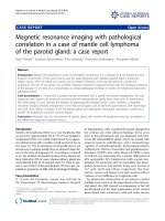
B

Figure 1-1 A: X-ray and B: computed tomography of head with cochlear implant. Note the
higher contrast of fine structures in the computed tomography slice, whereas superposition of
structures in the x-ray confounds the three dimensional location.

As a curious consequence of this progress, the very large
volume of image data acquired with current scanning techniques poses another challenge for interpretation: how to
display very large amounts of information for the interpretation process. The magnitude and complexity of true volume imaging requires new rendering techniques to enable
productive exploitation of the vast amount of information.

1 second, with reconstruction computations requiring several seconds per slice. Nevertheless, the time required to
scan a patient volume of interest often was longer than a
single breath-hold, and scan range was limited by x-ray tube
heat load to 10 to 30 cm. By translating the patient table
continuously through the rotating gantry, termed helical or
spiral scanning, volume coverage and scan speed were further
increased, with fundamental rate limitations being x-ray

Brief History of Computed Tomography
Evolution of CT Performance
108
107
Acquired Pixels per Second

Since its introduction in the mid-1970s, CT scanner technology has undergone a continual improvement in performance, including increases in acquisition speed,
amount of information in individual slices, and volume
of coverage. A graph (Fig. 1-2) of these parameters versus
time looks similar to Moore’s Law for computer priceperformance, which observes that computer metrics
(clock speed, cost of random access memory or magnetic storage, etc.) double every 18 months. In the case
of CT technology, the doubling period is approximately
32 months, still an impressive rate. For example, scan

time per slice has decreased from 300 seconds in 1972 to
0.005 seconds in 2005. Factors contributing to this remarkable advance include improvements in electronics
hardware and development of innovative mechanical
scanning configurations.
Historically, the early scanner configurations were characterized as successive generations of scanner geometry
(Fig. 1-3). By 1990 rotating fan beam systems, utilizing
slip-ring technology to allow continuous rotation of x-ray
tube and detector, had reduced acquisition time to about

106
105
104
103
102
1970

1975

1980

1985 1990
Date

1995

2000

2005

Figure 1-2 Evolution of computed tomography scanner performance: plot of acquisition performance versus time, for computed

tomography scanners. The slope implies a doubling of performance
approximately every 2 years. (Data from Siemens Medical Systems,
www.medical.siemens.com, “CT History and Technology.”)


5063_Lee_Ch01pp0001-0028 10/13/05 12:01 PM Page 3

Basic Principles of Computed Tomography Physics and Technical Considerations
1st generation (1970)

3

2nd generation (1972)
1. translation

translation
start

end

start
end

Pencil beam: translation/rotation

Partial fan beam: translation/rotation

3rd generation (1976)

4th generation (1978)

rotating detector arc

Fan beam: continuous rotation

stationary
detector ring
Fan beam: continuous rotation

tube output and mechanical rotation rate. Image reconstruction techniques were developed to interpolate 2D
planes from the 3D datasets that were acquired in helical
mode. In the late 1990s, the obstacles encountered by
early helical scanners were overcome by multidetector row
technology, using multiple sets of detector rows to utilize
more of the x-ray tube output and acquire measurements
at multiple section levels in parallel. Reconstruction under
these conditions is inherently 3D, so more complex algorithms must be used. Benefiting from substantial improvements in computing power, the rapid increases in CT
performance appear to be sustainable into the new century,
with development of flat panel detectors, faster electronics,
and cone-beam geometry reconstruction algorithms.
To understand best how to utilize CT technology clinically and appreciate new product capabilities, knowledge

Figure 1-3 Definition of the different generations of scan geometries.

of fundamental CT imaging principles is necessary. The
basic principles of CT involve physical mechanisms that
are shared with x-ray imaging, plus mathematical techniques
that exceed the human visual perception of 2D images. A
common technical description can be used to describe
both the image formation process and the image visualization task. These will now be examined in detail.

COMPUTED TOMOGRAPHY
ACQUISITION SYSTEM COMPONENTS
Generation of X-Rays
For medical imaging, x-rays are generated by an x-ray tube.
In this device, a metal filament is heated (much like a light
bulb) until energetic electrons escape from the cathode


5063_Lee_Ch01pp0001-0028 2/17/06 9:37 AM Page 4

4

Chapter 1
0.08
0.07

Probability

0.06
0.05
0.04
0.03
0.02
0.01
0

100

50

150

Energy (keV)

Figure 1-4 Typical x-ray spectrum for tungsten target with
120 kVp. Low-energy photons, which do not pass through the
patient to contribute to final image, have been filtered out.

surface into a vacuum. These electrons are then accelerated by an electric field, acquiring kinetic energy while
being attracted to a positive anode target. The total
amount of energy acquired by the electron in the accelerating electric field is equal to the product of the potential
(peak kilovoltage, kVp) times the unit of electrical charge,
possessing units of electron volts (kilo electron volts, keV).
The amount of charge generated by the x-ray tube per unit
time has units of electrical current (milliamperes, mA),
and the product of voltage and current is the amount of
power (watts) delivered by the tube. Electrostatic and/or
magnetic fields are used to focus the electron beam into a
small area of the anode target. Typically, this focal spot has
dimensions of about 1 mm. When the electrons collide
with the target, most of their energy is dissipated into heat
but a small fraction (Ͻ1%) is converted into several forms
of electromagnetic radiation. A typical spectrum of the distribution of energy emitted by the x-ray tube is shown in
Figure 1-4. Characteristically, there is a linearly decreasing
portion caused by bremsstrahlung, the deceleration of the
electrons in the target. According to Maxwell’s equations,
any charge undergoing acceleration will radiate electromagnetic energy. As beam electrons pass through target
atoms, they interact and are accelerated. The maximum
amount of energy that can be transferred is equal to

e ϫ kVp, and lesser amounts of energy appear randomly
depending on the details of electron collisions. The sharp
peaks in the spectrum occur when the beam electrons deposit energy by exciting atomic electrons in the target.
Electron shell transfers arise in atoms, with characteristic
radiation at well-defined (K-edge) energy peaks.
The spectrum generated in an x-ray tube contains many
low energy photons. The power in the beam associated
with a particular energy range is fairly constant, because
the number of quanta decreases linearly as a function of

energy, while the energy of an individual quantum increases linearly. Because the lowest energy quanta are effectively attenuated in the patient, they contribute very little
to the measured signal while exposing the patient to radiation dose. Therefore, the beam is filtered by placing material
around the x-ray tube to reduce much of the low energy
quanta while passing high energy quanta, leading to an
optimal image quality/dose tradeoff.
The x-rays from the target are spread over a wide solid
angle (essentially a hemisphere). To minimize radiation
dose and generation of background scatter, the x-ray beam
is collimated by an aperture into a thin fan beam. For CT
scanners, the beam is typically a few millimeters thick in
the patient, subtending a fan of about 45 degrees. Additionally, because human anatomy typically has a round
cross-section that is thicker in the middle than in the periphery, more x-ray flux reaches detectors on the edges
than at the center. This means that patients receive more
dose than is necessary on the periphery of their anatomy.
To compensate for this effect, a bowtie-shape filter is
placed in the beam, which is tapered such that its center is
thinner than its edges, to equalize the flux reaching the detectors and minimize patient dose.
The inefficiency in conversion of electron current into
x-rays has been a significant practical limitation in the operation of x-ray imaging equipment. The tube is quickly
heated to high temperatures, which must be limited to

avoid damage. Anode targets have been designed to rotate
on bearings, spreading out the area that is heated by the
beam. Heat sinks are used to remove heat from the system
by convection or water-assisted cooling.
In typical clinical operation, an x-ray tube delivers on
the order of 2 ϫ 1011 x-rays per second to the patient, providing a high signal-to-noise ratio for measurements.

Detection of X-Rays
Detection of x-rays is accomplished by the use of special
materials that convert the high energies (tens of keV) of
the x-ray quantum into lower energy forms, such as optical
photons or electron-hole pairs, which have energies of a
few electron volts. In this down-conversion, many secondary quanta are generated, typically thousands per primary
quanta. The detector materials, such as phosphors, scintillating ceramics, or pressurized xenon gas, ultimately produce an electrical current or voltage. Electronic amplifiers
condition this signal, and an analog-to-digital converter
converts it into a digital number. The range of signals produced in tomography is large, varying from a scan of air
(no attenuation, or 100% transmission) to that of a large
patient with metal implants (possible attenuation of
0.0006%), a factor of almost 105. Furthermore, even at the
lowest signal levels, the analog-to-digital converter must be
able to detect modulations of a few percent. Thus the overall range approaches a factor of one million, specifying the
equivalent of a 20-bit analog-to-digital converter.


5063_Lee_Ch01pp0001-0028 10/13/05 12:01 PM Page 5

Basic Principles of Computed Tomography Physics and Technical Considerations

Gantry Electromechanics
To obtain required measurements at different angles, all

the electrical components must be rotated around the patient. In modern scanners, this puts tremendous requirements on mechanical precision and stability. The gantry
can weigh 400 to 1,000 kg, span a diameter of 1.5 m, and
rotate 3 revolutions per second. While rotating, it may not
wobble more that 0.05 mm.
Originally, the gantry was connected by cables to the
outside environment and had to change rotation direction
at the end of each revolution. A major breakthrough in
scanning operation occurred with the invention of slip-ring
technology, which used brush contacts to provide continuous electrical power and electronic communication, allowing continuous rotation.

Helical/Spiral Scanning
One of the primary goals of CT manufacturers has been to
provide faster scan times and larger scan coverage. With
the advent of slip-ring technology and continuous gantry
rotation, the main limitation to scanning speed was the
stepping of the patient bed to position sequential slices. In
the late 1980s continuous motion of the patient table was
introduced, which allowed faster scan times but required
different data handling for image reconstruction (Fig. 1-5).
Previously the theory of CT reconstruction was based on
having a complete set of gantry measurements for each
slice reconstructed. However, in helical scans the gantry is
at continuously different table positions throughout each
rotation. A good mathematical approximation for each
gantry position is to interpolate a reconstruction plane
from corresponding neighboring gantry positions. This
approach provided adequate image quality, and in fact had
the added benefit that slices could be reconstructed retrospectively for arbitrary table positions, instead of being
limited to fixed table increments. Furthermore, analysis revealed that on average the spatial resolution was better

5

with helical scans rather than sequential scans. A drawback
was that the interpolation process could create stair-step
artifacts on the boundaries of extended high-contrast objects.

Detector Configuration
By the mid-1990s, helical scans had become limited in
speed because of the mechanical forces associated with
subsecond gantry rotation times and the output requirements of x-ray tubes to supply enough flux for adequate
signal to noise ratio. The next improvement in performance resulted from acquiring measurements at multiple
body levels in parallel, using more than one row of detectors at the same time. This advance allowed an increase in
speed of volume acquisition proportional to the number
of rows of detectors. In this approach, the x-ray tube produces a broad beam of x-rays, rather than one that is collimated to a narrow slice; by widening the collimation to illuminate multiple rows of detectors, more measurements
are acquired from the same tube output. Initially, two- or
four-row multidetector row CT (MDCT) scanners were introduced, but the number of detector rows has grown
steadily, with 64-detector row devices now enabling very
large volume coverage. Because of the increased longitudinal width of the x-ray beam with MDCT, image data measurements no longer correspond to rays orthogonal to the
scan axis; thus new reconstruction algorithms are required
to maintain image quality and prevent distortions.
In single-detector row CT (SDCT), each individual detector row functions as a single unit and provides projection data for a single section per rotation. In SDCT, different section widths are obtained by means of adjusting
prepatient collimation of the x-ray beam (Fig. 1-6). In
MDCT, the detectors are further divided along the z-axis,
allowing simultaneous acquisition of multiple sections per
rotation. Thus MDCT provides larger and faster z-axis coverage per rotation with thinner section widths.

Path of continuously
rotating x-ray tube
and detector

Start
spiral scan

Direction of
patient transport
0
Start
0

z, mm
t, s

Figure 1-5 Helical or spiral scanning involves translating the patient
longitudinally through the rotating
gantry.


5063_Lee_Ch01pp0001-0028 10/13/05 12:01 PM Page 6

6

Chapter 1
Focus

X-ray focus

Collimator

Scan-FOV

Scanfield
16x1.25

z-axis

z-axis

Fixed Array
Detector

Detector

A

X-ray focus
5

2.5

1.5

1

1

1.5

X-ray focus
2.5

5

Scanfield

Scanfield
4x1.5

z-axis

16x0.75

4x1.5

Adaptive
Array Detector

C

B

16 rows, 4 slices

Slice-Width

8 rows, 4 slices

24 rows, 16 slices

z-axis

Adaptive
Array Detector D

Figure 1-6 Multidetector computed tomography configurations. A: Illustration shows prepatient
collimation of the x-ray beam to obtain different collimated section widths with a single-detector
row computed tomography detector. FOV ϭ field of view. Illustrations show examples of (B) fixedarray and (C, D) adaptive-array detectors used in commercially available four-section and 16-section
computed tomography systems.

When four-channel MDCT scanners were introduced in
the late 1990s, three different detector configurations were
used by the CT manufacturers: (A) 16 detector rows with a
uniform thickness, termed uniform array (General Electric);
(B) eight detector rows of variable thicknesses, thinner
rows centrally and wider rows peripherally, termed adaptive
array [Siemens and Philips]; and (C) 34 detector rows with
two fixed thicknesses, four thinner rows centrally and 30
thicker rows peripherally, termed hybrid array (Toshiba).
Note that four-channel MDCT systems contain detectors
that are divided into eight to 34 rows along the z-axis. Nevertheless, the number of sections acquired at each rotation
is restricted to four because these systems contain only
four data channels. When a scan with a narrow collimation is desired, four individual central detector rows are
used for the data measurement, with a narrowly collimated x-ray beam directed over these central detector rows
(e.g., 4 ϫ 1 mm). To generate scans with larger section
widths, a broadly collimated x-ray beam is used, and outputs from two or more adjacent detector rows are electronically combined into a single thicker detector row for each
of the four data channels. For example, two 1-mm detector
rows can be grouped to function as a single detector row
for 2-mm collimation (4 ϫ 2 mm), three 1-mm detector
rows for 3-mm collimation (4 ϫ 3 mm), and so on.

For 16-channel MDCT, all of the CT manufacturers

adopted a hybrid array design, in which the thickness of the
detector rows is slightly less than 1 mm for the central
rowsand slightly more than 1 mm for the peripheral rows.
However, the length of the z-axis coverage and the number
of detector rows varies widely among the CT manufacturers.
For 64-channel MDCT, the CT manufacturers have
again used a common detector row design, this time a uniform array in which all the detector rows have a uniform
thickness. However, as in 16-channel MDCT, the total
number of detector rows and the z-axis coverage are highly
variable among the CT manufacturers.

COMPUTED TOMOGRAPHY
IMAGE FORMATION
X-Ray Signals
X-ray imaging consists of the generation of x-rays, transmission of those x-rays through material objects, and the
detection of the beam energy that exits the object. The attenuation of x-rays within an object is governed by interactions on the atomic scale, in which each molecule in the
object has some cross section for interacting with each x-ray.
Because of this interaction, the x-ray flux decreases on


5063_Lee_Ch01pp0001-0028 2/17/06 9:37 AM Page 7

Basic Principles of Computed Tomography Physics and Technical Considerations

average by a certain percentage for each unit distance traveled
through the object. Thus, if a 60 keV x-ray travels through
1 mm of water, on average it will survive 97.4% of the time.
For 2 mm of water, the survival probabilities multiply for a
95% rate. The transmission probability is thus an exponentially decreasing function of the total amount and type of
material present, represented by Lambert-Beer equation:

S ϭ I expaϪa ␮iti b

(1)

i

where S is the number of surviving signal quanta, I is the
number of incident quanta, the subscript i indicates different materials that are compose the sample, ␮i is the linear
attenuation coefficient for each material and ti is the
amount (thickness) of that material present.
In projection x-ray imaging, the image consists of the relative changes in the signal S across a viewing area. For a 70-kg
person, with an abdomen roughly equivalent to 20-cm
thickness of water, the survival probability for a single quantum would be about 2%. The presence of an additional 2 mm
of abnormal structure would change this survival probability
to 1.98% (only a 1% difference). Given this small change in
the midst of many overlapping body structures, it is clear
that projection radiography is limited in its ability to
demonstrate anatomic details. In CT imaging, measurements
of S are made from multiple projections, and from these
measurements ␮i is computed for direct display. This technique results in much higher relative contrast between adjacent
structures. For example, a 2-mm calcified nodule may have a
200% difference in attenuation coefficient compared with
surrounding tissue, and hence be much more conspicuous
than on a projection radiograph (see Fig. 1-1).
For the viewing of images, projection x-rays are presented as a brightness that is proportional to the changes
of the transmitted signal S in Eq. 1. In CT, the image attenuation map is presented in units that are relative to the attenuation coefficient of water, expressed as Hounsfield
units (HU).
␮i Ϫ ␮water
HUi ϵ 1,000
(2)

␮water

7

Image Reconstruction From Two-Dimensional
Projection Data
The basics of CT image generation can be illustrated by the
reconstruction of a 2D image section from projection
measurements. An x-ray source and a set of detectors rotate
around the patient, making measurements of the transmission of x-rays through the body. Each measured value is the
result of all the attenuating portions in the patient along a
line from the x-ray source to the detector making the measurement. Hence, a uniform circular disk will have highest
attenuation in its center, with a circular profile. The collection of line measurements from different view angles during
one revolution of the gantry provides raw projection data
prior to reconstructing images. The raw projection data
result in a sinogram (Fig. 1-7). The sinogram can be displayed as an image, with the y-axis (rows) representing the
measurements of each detector and the x-axis (columns)
representing detector measurements at one gantry position. The sinogram image has an intriguing pattern, but is
difficult to interpret because of the overlapping shapes.
Thus, a method is needed to derive and compute the original image attenuation.
One method, albeit impractical, for determining the
source image involves treating the sinogram and image as
a linear algebra problem. Each measurement is an equation summing all the image pixels along a ray to the detector; the set of all equations can then be solved for the
image pixel unknowns. The size of this problem is dauntingly large because there are 512 ϫ 512 (i.e., more than
one quarter million) variables involved with 768 ϫ 1,400
(i.e., more than one million) measurements, requiring matrix operations that overwhelm even modern computers.
Other mathematical methods, such as iterative techniques
or maximum likelihood optimization, can be used to
solve for images, but they also are too computationally intensive for routine clinical usage.
The mathematical process that made CT reconstruction

practical is called filtered back projection. It can be shown
theoretically (18) that if the projection measurements
have certain properties (they all lie in one plane, they con-

A

B
Figure 1-7 An abdominal slice and its sinogram.


5063_Lee_Ch01pp0001-0028 2/17/06 9:37 AM Page 8

8

Chapter 1

sist of equally spaced gantry steps covering at least one half
revolution, and the detectors are equidistant and cover the
whole object to be reconstructed), then the attenuation
(image) at any point within the scanner field of view can
be calculated by summing a certain weighted combination
of the measurements. This weighted summation process is
called a kernel (see the section titled Reconstruction Kernel
later in this chapter for detail). The measurement of the detector directly intercepting the pixel is added and measurements from neighboring detectors are subtracted. Different
kernels can be designed to provide sharp, crisp images or to
smooth out noise, depending on the clinical application.
This process, which was universally adopted by CT manufacturers in the early years of CT, can be performed very efficiently by computers or special hardware modules, either
directly or with Fast Fourier Transform techniques.

Image Reconstruction from

Three-Dimensional Projection Data
The filtered back projection process requires that the
image data be confined to a single plane. With helical CT,
3D volumes rather than single sections of data are acquired, necessitating the development of new reconstruction algorithms.

Single-Detector Row Spiral Computed
Tomography: Linear Interpolation
In spiral scanning, the patient table moves continuously,
so at any given longitudinal or z-location there are only a
few (or no) exactly corresponding gantry measurements
that are aligned in the same plane for 2D filtered back projection. The higher the pitch (i.e., the faster the CT table
travels relative to the detector collimation), the more the
gantry measurements separate and deviate from the plane.
To provide a complete set of measurements for filtered
back projection, missing gantry measurements are estimated by taking the average of the closest (in the z-axis)
measurements that are collected.
Two versions of this method are employed. The first is
called 360LI and takes averages of measurements separated
by one rotation. In this approach, to generate projection
data for a target image plane, two gantry measurements on
either side of the image plane that are positioned closest to
the image plane and are 360 degrees apart (i.e., are measured in subsequent rotations) are linearly interpolated for
each projection angle. The 360LI technique has the disadvantage that the travel in one revolution may be large, and
if structures change significantly over this distance blurring
or partial volume averaging will result.
The second method, called 180LI, takes advantage of
the symmetry between x-ray source and detector across
the gantry, i.e., the measured ray is nominally the same
when the source-detector positions are one half rotation
(180 degrees) apart. The 180LI technique makes use of

the fact that for each measurement ray, an interpolation

partner is already available after approximately one half a
rotation, when the x-ray tube and detector have switched
positions. This virtual, geometrically derived ray is called a
complementary ray. The 180LI technique involves smaller
z-distances and hence suffers less blurring. (The same trick
can be used in cardiac imaging, to shorten the time window
for an image snapshot and minimize temporal blur.)

Multidetector Row Spiral Computed Tomography:
Z-Interpolation or Z-Filtering
The first multidetector row scanners had two or four detector rows, and the data measurements could be treated as a
simple parallel stack of independent detector rows. In this
case, the 360LI and 180LI used in SDCT spiral reconstruction approaches can be directly extended to spiral MDCT.
One could then create planes of measurements by linear
interpolation (either 360LI or 180LI) from the closest row
measurements to the target plane, a technique known as
advanced single-slice rebinning (16). The interpolation calculation can be performed very rapidly and is essentially
similar to single-row scanning. In the 360LI interpolation
approach, the interpolation can be performed using rays
measured at the same projection angle by different detector
rows or in consecutive rotations of the scanner 360 degrees
apart. In the 180LI reconstruction approach, both direct
and complementary rays can be used for spiral interpolation.
CT scanner manufacturers proposed different mathematical
approaches for weighting and interpolating neighboring
rays for the target image plane, such as z-interpolation or
z-filtering (17,32,34).

Broad Beam Multidetector or Flat-Panel Computed
Tomography: Cone Beam Reconstruction
With increases in the number of detector rows beyond
four, it becomes necessary to account for the cone-beam
angle between detector rows (8). Some manufacturers use
variations and extensions of nutating-section algorithms
for image reconstruction (4,16,21,31). These algorithms
split the 3D reconstruction task into a series of conventional 2D reconstructions on tilted intermediate image
planes, thereby benefiting from established and very fast
2D reconstruction techniques. Examples are adaptive multiplanar reconstruction (Siemens) (7) and the weighted
hyperplane reconstruction (GE Medical Systems) (12) techniques. Other manufacturers (Toshiba, Philips) have extended to multisection scanning the Feldkamp algorithm
(6,9), an approximate 3D convolution back-projection reconstruction that was originally introduced for sequential
scanning. With this approach, accounting for their conebeam geometry, the measurement rays are back projected
into a 3D volume along the lines of measurement. Three-dimensional back projection is, however, computationally
demanding and requires dedicated hardware to achieve acceptable image-reconstruction times. The development of
methods to account for the cone-beam geometry of the
measurement x-rays currently is an active area of research.


5063_Lee_Ch01pp0001-0028 10/13/05 12:01 PM Page 9

Basic Principles of Computed Tomography Physics and Technical Considerations

IMAGING METRICS
Although image quality is the ultimate measure of an imaging system, it is difficult to define and quantify image
quality. In clinical settings, image quality is frequently determined qualitatively and subjectively. Communication
theory specifies the fundamental parameters of information transfer as signal, resolution, distortion, and noise to
characterize system performance. Several quantitative and
objective parameters are commonly used to describe
image quality: spatial resolution, contrast resolution, temporal

resolution, noise, and artifacts. These parameters are affected
by CT scanner apparatus and scan variables and are often
used to assess the performance of a CT scanner.

Signal
An image represents a map of some physical quantity, either
directly measured or derived from measurements. The
image signal can be continuous, as in a screen-film x-ray or
35-mm photograph, or they can be discrete, such as a
medical image on a computer monitor. In the CT acquisition process, the quantity measured is the attenuation of
the x-ray beam (just like a projection x-ray), with a continuous physical electrical signal representing x-ray energy
flux, converted to a discrete digital value. From a set of
these measurements, a digital image is calculated to represent the attenuation coefficient of the material in the object. The map is a collection of pixels (picture elements),
typically a square array of 512 pixels on a side. When multiple slices are collected into volume data sets, the 3D map
becomes a collection of voxels (volume elements). In computer terms, the original measurements may consist of 16bit data (allowing a range of values spanning a factor of
64,000), whereas the reconstructed images typically are 8or 12-bit data (a range up to 4,095). It is assumed that the
signal is linear with the physical properties of the displayed object. For example, if the density of the contrast
medium in a voxel doubles, the pixel value will increase by
a factor of two.
The information in the image signal consists of patterns
of change in the image. The magnitude of such change is
characterized by contrast, the variation of local values
from the surrounding values. In discrete, digital systems,
the bit depth of the data determines the smallest change
recordable, typically 0.02% step (12 bits) in the digital
data or 0.4% step (8 bits) for a displayed image.
In the image display process, signal relates to the intensity of light patterns that a human observer views. The dynamic range of light signal may be a factor of 500 to
Ϫ1,000 from light to dark. Signals can be transformed into
different representations, e.g., a CT attenuation image file
gets mapped to a light intensity signal for viewing on a

monitor, with brightness and contrast adjustments to emphasize different areas of interest.

9

Resolution
The term resolution characterizes the ability of an imaging
system to detect changes in a signal; the term arises in several different contexts in image operations (e.g., spatial or
temporal resolution). The ability of an imaging system to
record changes between different points in space depends
on two factors: system aperture and (for discrete systems)
sampling rate. A system aperture can take different forms:
in a display system, it may be the size of the spot of light to
form the image; in a CT scanner, it could be the size of the
detector cell that measures the x-ray flux. The aperture is
considered piece-wise constant within itself, so changes
can only be recorded over a size commensurate with its dimensions. Spatial resolution is characterized by a point
spread function, which is the signal footprint of an infinitesimal size (point) input, and is expressed as length (such
as full-width at half maximum value of the point spread
function). Equivalently, the resolution can be reported in
the frequency domain by describing a modulation transfer
function (MTF), which characterizes how signals of different spatial frequencies (size) are attenuated by the measuring system.
In discrete systems, an additional factor affecting resolution is the sampling rate at which signals are transferred.
For example, a moving light beam 1 mm in diameter
might be modulated every 0.5 mm. Elegant mathematical
analyses exist for describing the effect of sampling rate on
signal information. One often used result is the Nyquist
criterion, which states that at least two samples are required over the distance of the system aperture to prevent
distortion of signal information. Such analysis is used extensively in designing medical imaging systems.

Spatial (High-contrast) Resolution

Spatial resolution measures the capability of an imaging
system to resolve closely placed objects or to display fine
details. The spatial resolution of CT is described in two dimensions, xy-image (in-plane) resolution and z-direction
(longitudinal) resolution. In-plane and longitudinal resolution depend on different factors. Traditionally the in-plane
spatial resolution has been far better than the longitudinal
or cross-plane spatial resolution, but the longitudinal resolution has been significantly improved with MDCT and
approaches that of the in-plane resolution.

In-Plane Spatial Resolution
In-plane spatial resolution is usually expressed in line
pairs per millimeter, typically 0.5 to 2 lp/mm for CT. It is
often measured directly by imaging and visualizing highcontrast objects of increasingly smaller sizes or increasing
spatial frequencies (Fig. 1-8). However, the evaluation
process involved in this approach may be subjective. More
objective, quantitative methods are based on calculation of
MTF, which is defined as the ratio of the output modulation to the input modulation, measuring the response of


5063_Lee_Ch01pp0001-0028 2/17/06 9:38 AM Page 10

10

Chapter 1

Figure 1-8 Bar targets used to determine resolution (from
Siemens Medical Systems).

an imaging system to different frequencies. The MTF is
most commonly obtained by taking a Fourier transformation of the point spread function that is measured by scanning the cross-section of a thin wire phantom. It is expressed by a plot of the fraction of subject contrast in the
image versus spatial frequency. Spatial resolution is then

specified at the frequency for a given percent value of the
MTF (Fig. 1-9).
The spatial resolution of a CT imaging system depends
on the quality of raw CT projection data and the reconstruction method. The spatial resolution of the projection
data is in turn influenced by system geometric resolution
limits such as focal spot size, detector width, and x-ray
beam sampling. After a CT scan is acquired, the spatial resolution of the reconstructed CT image can be affected by
the selection of a field of view or zoom factor. With the use
of a small field of view, the size of the individual pixels decreases and the in-plane spatial resolution of a CT image
increases.

Longitudinal Spatial Resolution
(Slice Sensitivity Profile)
The longitudinal spatial resolution is usually expressed
by slice sensitivity profile (SSP),which describes the longitudinal profile of a CT scanner point spread function
(Fig. 1-10). The SSP is measured using small thin
platelets, just as a thin wire phantom is used to measure
the point spread function for the in-plane resolution. The
profile is typically a Gaussian curve shape, blurred from
the ideal rectangular shape. In spiral CT, the SSP broadens because of the movement of the CT scanner table
during the CT gantry rotation. From the SSP, the longitudinal resolution is generally characterized by two numbers: the full width at half maximum or full width at
tenth maximum.

The longitudinal resolution has become increasingly
important in view of the increasing application of volume
examinations and 3D representation. In sequential (SDCT
or MDCT) scanning, the SSP is readily defined and mainly
determined by x-ray beam collimation. In spiral (SDCT or
MDCT) scanning, however, the SSP becomes more complex depending on multiple other factors such as the CT
table speed (pitch), spiral interpolation algorithm, detector width (especially in MDCT), and crosstalk between

neighboring slices. For spiral SDCT, a higher table speed
results in a broader SSP and thus a larger effective slice
thickness. The 180LI interpolation algorithm produces
thinner SSP than the 360LI algorithm at the cost of higher
noise (29,30). For spiral MDCT, the relationship between
the table speed (i.e., pitch) and SSP is less straightforward,
because multiple sets of spiral data collected from multiple detectors can be interpolated in more complex fashions (25). (See the section titled Computed Tomography
Table Travel Speed and Pitch later in this chapter for more
detail on the effect of table speed.) With MDCT, variations
among CT manufacturers in hardware implementation
and algorithmic approaches make it difficult to provide
general statements about the effect of scan factors on longitudinal resolution.

Contrast (Low-contrast) Resolution
Low-contrast resolution of an image system is the ability
to distinguish a low-contrast object from its background.
This is a property in which CT is far superior to conventional radiographs. Low-contrast resolution is measured
using phantoms that contain objects of varying sizes
with small difference in attenuation value from background (Fig. 1-11). The most widely accepted methods of
measuring low-contrast resolution of a system are based
on the subjective response of an observer to detect objects as
distinct. Because the difference between object and background signal is small, noise plays an important role in
determining low-contrast resolution. Many factors that influence the noise level such as tube current, tube voltage,
slice thickness, and reconstruction algorithm also affect
low-contrast resolution. In addition to these factors, the
size of objects and viewing window setting also affect lowcontrast detectability. In CT, the contrast difference between objects is typically characterized by the percentage
linear attenuation coefficient: 1% contrast difference corresponds to a difference of 10 HU.

Temporal Resolution
Temporal resolution determines how rapidly changing signals can be recorded. As CT technology advances, temporal resolution increases continuously with an increase in

volume coverage and scan speed. High temporal resolution is particularly desirable when imaging moving structures (e.g., heart, lungs) and for dynamic contrast medium