Ebook Operating systems - Internals and designprinciples (9/E): Part 2

www.downloadslide.net

Part 5 Input/Output and Files
Chapter

I/O Management and Disk
Scheduling
11.1
11.2

I/O Devices
Organization of the I/O Function
The Evolution of the I/O Function
Direct Memory Access
11.3 Operating System Design Issues
Design Objectives
Logical Structure of the I/O Function
11.4 I/O Buffering
Single Buffer
Double Buffer
Circular Buffer
The Utility of Buffering
11.5 Disk Scheduling
Disk Performance Parameters
Disk Scheduling Policies
11.6 RAID
RAID Level 0
RAID Level 1
RAID Level 2
RAID Level 3
RAID Level 4

RAID Level 5
RAID Level 6
11.7 Disk Cache
Design Considerations
Performance Considerations
11.8 UNIX SVR4 I/O
Buffer Cache
Character Queue
Unbuffered I/O
UNIX Devices
11.9 Linux I/O
Disk Scheduling
Linux Page Cache
11.10 Windows I/O
Basic I/O Facilities
Asynchronous and Synchronous I/O
Software RAID
Volume Shadow Copies
Volume Encryption
11.11 Summary
11.12 Key Terms, Review Questions, and Problems

M11_STAL4290_09_GE_C11.indd 505

505

5/9/17 4:32 PM


www.downloadslide.net

506   Chapter 11 / I/O Management and Disk Scheduling
Learning Objectives
After studying this chapter, you should be able to:
• Summarize key categories of I/O devices on computers.
• Discuss the organization of the I/O function.
• Explain some of the key issues in the design of OS support for I/O.
• Analyze the performance implications of various I/O buffering alternatives.
• Understand the performance issues involved in magnetic disk access.
• Explain the concept of RAID and describe the various levels.
• Understand the performance implications of disk cache.
• Describe the I/O mechanisms in UNIX, Linux, and Windows.

Perhaps the messiest aspect of operating system design is input/output. Because there
is such a wide variety of devices and applications of those devices, it is difficult to
develop a general, consistent solution.
We begin with a brief discussion of I/O devices and the organization of the I/O
function. These topics, which generally come within the scope of computer architecture, set the stage for an examination of I/O from the point of view of the OS.
The next section examines operating system design issues, including design
objectives, and the way in which the I/O function can be structured. Then I/O buffering is examined; one of the basic I/O services provided by the operating system is a
buffering function, which improves overall performance.
The next sections of the chapter are devoted to magnetic disk I/O. In contemporary systems, this form of I/O is the most important and is key to the performance
as perceived by the user. We begin by developing a model of disk I/O performance
then examine several techniques that can be used to enhance performance.
Appendix J summarizes characteristics of secondary storage devices, including
magnetic disk and optical memory.

  11.1 I/O DEVICES
As was mentioned in Chapter 1, external devices that engage in I/O with computer
systems can be roughly grouped into three categories:
1. Human readable: Suitable for communicating with the computer user. Examples include printers and terminals, the latter consisting of video display, keyboard, and perhaps other devices such as a mouse.

2. Machine readable: Suitable for communicating with electronic equipment.
Examples are disk drives, USB keys, sensors, controllers, and actuators.
3. Communication: Suitable for communicating with remote devices. Examples
are digital line drivers and modems.

M11_STAL4290_09_GE_C11.indd 506

5/9/17 4:32 PM


www.downloadslide.net
11.1 / I/O DEVICES   507
Gigabit ethernet
Graphics display
Hard disk
Ethernet
Optical disk
Scanner
Laser printer
Floppy disk
Modem
Mouse
Keyboard
101

102

103

104

105
Data Rate (bps)

106

107

108

109

Figure 11.1  Typical I/O Device Data Rates

There are great differences across classes and even substantial differences
within each class. Among the key differences are the following:
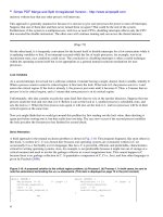
• Data rate: There may be differences of several orders of magnitude between
the data transfer rates. Figure 11.1 gives some examples.
• Application: The use to which a device is put has an influence on the software and policies in the OS and supporting utilities. For example, a disk used
for files requires the support of file management software. A disk used as a
backing store for pages in a virtual memory scheme depends on the use of
virtual memory hardware and software. Furthermore, these applications have
an impact on disk scheduling algorithms (discussed later in this chapter). As
another example, a terminal may be used by an ordinary user or a system
administrator. These uses imply different privilege levels and perhaps different
priorities in the OS.
• Complexity of control: A printer requires a relatively simple control interface. A
disk is much more complex. The effect of these differences on the OS is filtered
to some extent by the complexity of the I/O module that controls the device, as
discussed in the next section.

• Unit of transfer: Data may be transferred as a stream of bytes or characters
(e.g., terminal I/O) or in larger blocks (e.g., disk I/O).
• Data representation: Different data encoding schemes are used by different
devices, including differences in character code and parity conventions.

M11_STAL4290_09_GE_C11.indd 507

5/9/17 4:32 PM


www.downloadslide.net
508   Chapter 11 / I/O Management and Disk Scheduling
• Error conditions: The nature of errors, the way in which they are reported,
their consequences, and the available range of responses differ widely from
one device to another.
This diversity makes a uniform and consistent approach to I/O, both from the
point of view of the operating system and from the point of view of user processes,
difficult to achieve.

  11.2 ORGANIZATION OF THE I/O FUNCTION
Appendix C summarizes three techniques for performing I/O:
1. Programmed I/O: The processor issues an I/O command, on behalf of a process,
to an I/O module; that process then busy waits for the operation to be completed before proceeding.
2. Interrupt-driven I/O: The processor issues an I/O command on behalf of a process. There are then two possibilities. If the I/O instruction from the process
is nonblocking, then the processor continues to execute instructions from the
process that issued the I/O command. If the I/O instruction is blocking, then the
next instruction that the processor executes is from the OS, which will put the
current process in a blocked state and schedule another process.
3. Direct memory access (DMA): A DMA module controls the exchange of data
between main memory and an I/O module. The processor sends a request for

the transfer of a block of data to the DMA module, and is interrupted only after
the entire block has been transferred.
Table 11.1 indicates the relationship among these three techniques. In most
computer systems, DMA is the dominant form of transfer that must be supported by
the operating system.

The Evolution of the I/O Function
As computer systems have evolved, there has been a pattern of increasing complexity
and sophistication of individual components. Nowhere is this more evident than in
the I/O function. The evolutionary steps can be summarized as follows:
1. The processor directly controls a peripheral device. This is seen in simple microprocessor-controlled devices.
2. A controller or I/O module is added. The processor uses programmed I/O without interrupts. With this step, the processor becomes somewhat divorced from
the specific details of external device interfaces.
Table 11.1  I/O Techniques

I/O-to-Memory Transfer through
Processor
Direct I/O-to-Memory Transfer

M11_STAL4290_09_GE_C11.indd 508

No Interrupts

Use of Interrupts

Programmed I/O

Interrupt-driven I/O
Direct memory access (DMA)

5/9/17 4:32 PM


www.downloadslide.net
11.2 / ORGANIZATION OF THE I/O FUNCTION   509

3. The same configuration as step 2 is used, but now interrupts are employed. The
processor need not spend time waiting for an I/O operation to be performed,
thus increasing efficiency.
4. The I/O module is given direct control of memory via DMA. It can now move
a block of data to or from memory without involving the processor, except at
the beginning and end of the transfer.
5. The I/O module is enhanced to become a separate processor, with a specialized
instruction set tailored for I/O. The central processing unit (CPU) directs the
I/O processor to execute an I/O program in main memory. The I/O processor
fetches and executes these instructions without processor intervention. This
allows the processor to specify a sequence of I/O activities and to be interrupted
only when the entire sequence has been performed.
6. The I/O module has a local memory of its own and is, in fact, a computer in its
own right. With this architecture, a large set of I/O devices can be controlled,
with minimal processor involvement. A common use for such an architecture
has been to control communications with interactive terminals. The I/O processor takes care of most of the tasks involved in controlling the terminals.
As one proceeds along this evolutionary path, more and more of the I/O function is performed without processor involvement. The central processor is increasingly relieved of I/O-related tasks, improving performance. With the last two steps
(5 and 6), a major change occurs with the introduction of the concept of an I/O
­module capable of executing a program.
A note about terminology: For all of the modules described in steps 4 through
6, the term direct memory access is appropriate, because all of these types involve
direct control of main memory by the I/O module. Also, the I/O module in step 5 is
often referred to as an I/O channel, and that in step 6 as an I/O processor; however,
each term is, on occasion, applied to both situations. In the latter part of this section,

we will use the term I/O channel to refer to both types of I/O modules.

Direct Memory Access
Figure 11.2 indicates, in general terms, the DMA logic. The DMA unit is capable of
mimicking the processor and, indeed, of taking over control of the system bus just
like a processor. It needs to do this to transfer data to and from memory over the
system bus.
The DMA technique works as follows. When the processor wishes to read or
write a block of data, it issues a command to the DMA module by sending to the
DMA module the following information:
• Whether a read or write is requested, using the read or write control line
between the processor and the DMA module
• The address of the I/O device involved, communicated on the data lines
• The starting location in memory to read from or write to, communicated on the
data lines and stored by the DMA module in its address register
• The number of words to be read or written, again communicated via the data
lines and stored in the data count register

M11_STAL4290_09_GE_C11.indd 509

5/9/17 4:32 PM


www.downloadslide.net
510   Chapter 11 / I/O Management and Disk Scheduling

Data
count
Data lines

Data
register

Address lines

Address
register

Request to DMA
Acknowledge from DMA
Interrupt
Read
Write

Control
logic

Figure 11.2  Typical DMA Block Diagram

The processor then continues with other work. It has delegated this I/O operation to the DMA module. The DMA module transfers the entire block of data, one
word at a time, directly to or from memory, without going through the processor.
When the transfer is complete, the DMA module sends an interrupt signal to the
processor. Thus, the processor is involved only at the beginning and end of the transfer (see Figure C.4c).
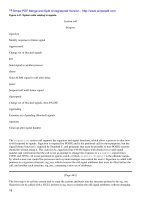
The DMA mechanism can be configured in a variety of ways. Some possibilities
are shown in Figure 11.3. In the first example, all modules share the same system bus.
The DMA module, acting as a surrogate processor, uses programmed I/O to exchange
data between memory and an I/O module through the DMA module. This configuration, while it may be inexpensive, is clearly inefficient: As with processor-controlled
programmed I/O, each transfer of a word consumes two bus cycles (transfer request
followed by transfer).
The number of required bus cycles can be cut substantially by integrating the

DMA and I/O functions. As Figure 11.3b indicates, this means there is a path between
the DMA module and one or more I/O modules that does not include the system bus.
The DMA logic may actually be a part of an I/O module, or it may be a separate module that controls one or more I/O modules. This concept can be taken one step further
by connecting I/O modules to the DMA module using an I/O bus (see Figure 11.3c).
This reduces the number of I/O interfaces in the DMA module to one and provides
for an easily expandable configuration. In all of these cases (see Figures 11.3b and
11.3c), the system bus that the DMA module shares with the processor and main
memory is used by the DMA module only to exchange data with memory and to
exchange control signals with the processor. The exchange of data between the DMA
and I/O modules takes place off the system bus.

M11_STAL4290_09_GE_C11.indd 510

5/9/17 4:32 PM


www.downloadslide.net
11.3 / OPERATING SYSTEM DESIGN ISSUES   511

Processor

DMA

I/O

Memory

I/O

(a) Single-bus, detached DMA

Processor

DMA

Memory

DMA

I/O
I/O

I/O

(b) Single-bus, integrated DMA-I/O
System bus

Processor

Memory

DMA

I/O bus

I/O

I/O

I/O

(c) I/O bus

Figure 11.3  Alternative DMA Configurations

  11.3 OPERATING SYSTEM DESIGN ISSUES
Design Objectives
Two objectives are paramount in designing the I/O facility: efficiency and generality.
Efficiency is important because I/O operations often form a bottleneck in a computing system. Looking again at Figure 11.1, we see that most I/O devices are extremely
slow compared with main memory and the processor. One way to tackle this problem
is multiprogramming, which, as we have seen, allows some processes to be waiting
on I/O operations while another process is executing. However, even with the vast
size of main memory in today’s machines, it will still often be the case that I/O is not
keeping up with the activities of the processor. Swapping is used to bring in additional
ready processes to keep the processor busy, but this in itself is an I/O operation. Thus,
a major effort in I/O design has been schemes for improving the efficiency of the I/O.
The area that has received the most attention, because of its importance, is disk I/O,
and much of this chapter will be devoted to a study of disk I/O efficiency.

M11_STAL4290_09_GE_C11.indd 511

5/9/17 4:32 PM


www.downloadslide.net
512   Chapter 11 / I/O Management and Disk Scheduling
The other major objective is generality. In the interests of simplicity and freedom from error, it is desirable to handle all devices in a uniform manner. This applies
both to the way in which processes view I/O devices, and to the way in which the OS
manages I/O devices and operations. Because of the diversity of device characteristics, it is difficult in practice to achieve true generality. What can be done is to use a
hierarchical, modular approach to the design of the I/O function. This approach hides

most of the details of device I/O in lower-level routines so user processes and upper
levels of the OS see devices in terms of general functions such as read, write, open,
close, lock, and unlock. We turn now to a discussion of this approach.

Logical Structure of the I/O Function
In Chapter 2, in the discussion of system structure, we emphasized the hierarchical
nature of modern operating systems. The hierarchical philosophy is that the functions of the OS should be separated according to their complexity, their characteristic time scale, and their level of abstraction. Applying this philosophy specifically
to the I/O facility leads to the type of organization suggested by Figure 11.4. The
details of the organization will depend on the type of device and the application.
The three most important logical structures are presented in the figure. Of course,
a particular operating system may not conform exactly to these structures. However, the general principles are valid, and most operating systems approach I/O in
approximately this way.
Let us consider the simplest case first, that of a local peripheral device that communicates in a simple fashion, such as a stream of bytes or records (see Figure 11.4a).
The following layers are involved:
• Logical I/O: The logical I/O module deals with the device as a logical resource
and is not concerned with the details of actually controlling the device. The
logical I/O module is concerned with managing general I/O functions on behalf
of user processes, allowing them to deal with the device in terms of a device
identifier and simple commands such as open, close, read, and write.
• Device I/O: The requested operations and data (buffered characters, records, etc.)
are converted into appropriate sequences of I/O instructions, channel commands,
and controller orders. Buffering techniques may be used to improve utilization.
• Scheduling and control: The actual queueing and scheduling of I/O operations
occurs at this layer, as well as the control of the operations. Thus, interrupts are
­handled at this layer and I/O status is collected and reported. This is the layer of
software that actually interacts with the I/O module and hence the device hardware.
For a communications device, the I/O structure (see Figure 11.4b) looks much
the same as that just described. The principal difference is that the logical I/O module
is replaced by a communications architecture, which may itself consist of a number
of layers. An example is TCP/IP, which will be discussed in Chapter 17.

Figure 11.4c shows a representative structure for managing I/O on a secondary
storage device that supports a file system. The three layers not previously discussed
are as follows:
1. Directory management: At this layer, symbolic file names are converted to
identifiers that either reference the file directly or indirectly through a file

M11_STAL4290_09_GE_C11.indd 512

5/9/17 4:32 PM


www.downloadslide.net
11.3 / OPERATING SYSTEM DESIGN ISSUES   513
User
processes

User
processes

User
processes

Directory
management

Logical
I/O

Communication
architecture

File system

Physical
organization

Device
I/O

Device
I/O

Device
I/O

Scheduling
& control

Scheduling
& control

Scheduling
& control

Hardware

Hardware

Hardware

(a) Local peripheral device

(b) Communications port

(c) File system

Figure 11.4  A Model of I/O Organization

descriptor or index table. This layer is also concerned with user operations that
affect the directory of files, such as add, delete, and reorganize.
2. File system: This layer deals with the logical structure of files and with the
operations that can be specified by users, such as open, close, read, and write.
Access rights are also managed at this layer.
3. Physical organization: Just as virtual memory addresses must be converted into
physical main memory addresses, taking into account the segmentation and
paging structure, logical references to files and records must be converted to
physical secondary storage addresses, taking into account the physical track
and sector structure of the secondary storage device. Allocation of secondary
storage space and main storage buffers is generally treated at this layer as well.
Because of the importance of the file system, we will spend some time, in this
chapter and the next, looking at its various components. The discussion in this chapter focuses on the lower three layers, while the upper two layers will be examined in
Chapter 12.

M11_STAL4290_09_GE_C11.indd 513

5/9/17 4:32 PM


www.downloadslide.net
514   Chapter 11 / I/O Management and Disk Scheduling

  11.4 I/O BUFFERING
Suppose a user process wishes to read blocks of data from a disk one at a time, with
each block having a length of 512 bytes. The data are to be read into a data area within
the address space of the user process at virtual location 1000 to 1511. The simplest
way would be to execute an I/O command (something like Read_Block[1000,
disk]) to the disk unit then wait for the data to become available. The waiting could
either be busy waiting (continuously test the device status) or, more practically, process suspension on an interrupt.
There are two problems with this approach. First, the program is hung up waiting
for the relatively slow I/O to complete. The second problem is that this approach to
I/O interferes with swapping decisions by the OS. Virtual locations 1000 to 1511 must
remain in main memory during the course of the block transfer. Otherwise, some of
the data may be lost. If paging is being used, at least the page containing the target
locations must be locked into main memory. Thus, although portions of the process
may be paged out to disk, it is impossible to swap the process out completely, even
if this is desired by the operating system. Notice also there is a risk of single-process
deadlock. If a process issues an I/O command, is suspended awaiting the result, and
then is swapped out prior to the beginning of the operation, the process is blocked
waiting on the I/O event, and the I/O operation is blocked waiting for the process to
be swapped in. To avoid this deadlock, the user memory involved in the I/O operation
must be locked in main memory immediately before the I/O request is issued, even
though the I/O operation is queued and may not be executed for some time.
The same considerations apply to an output operation. If a block is being transferred from a user process area directly to an I/O module, then the process is blocked
during the transfer and the process may not be swapped out.
To avoid these overheads and inefficiencies, it is sometimes convenient to perform input transfers in advance of requests being made, and to perform output transfers some time after the request is made. This technique is known as buffering. In this
section, we look at some of the buffering schemes that are supported by operating
systems to improve the performance of the system.
In discussing the various approaches to buffering, it is sometimes important
to make a distinction between two types of I/O devices: block-oriented and streamoriented. A block-oriented device stores information in blocks that are usually of
fixed size, and transfers are made one block at a time. Generally, it is possible to

reference data by its block number. Disks and USB keys are examples of blockoriented devices. A stream-oriented device transfers data in and out as a stream of
bytes, with no block structure. Terminals, printers, communications ports, mouse and
other pointing devices, and most other devices that are not secondary storage are
stream-oriented.

Single Buffer
The simplest type of support that the OS can provide is single buffering (see
­Figure 11.5b). When a user process issues an I/O request, the OS assigns a buffer in
the system ­portion of main memory to the operation.

M11_STAL4290_09_GE_C11.indd 514

5/9/17 4:32 PM


www.downloadslide.net
11.4 / I/O BUFFERING   515
Operating system
I/O device

User process

In

(a) No buffering
Operating system
I/O device

In

User process
Move

(b) Single buffering
Operating system
I/O device

In

User process
Move

(c) Double buffering
Operating system
I/O device

In

User process
Move

(d) Circular buffering

Figure 11.5  I/O Buffering Schemes (Input)

For block-oriented devices, the single buffering scheme can be described as follows: Input transfers are made to the system buffer. When the transfer is complete,
the process moves the block into user space and immediately requests another block.
This is called reading ahead, or anticipated input; it is done in the expectation that the
block will eventually be needed. For many types of computation, this is a reasonable
assumption most of the time because data are usually accessed sequentially. Only at

the end of a sequence of processing will a block be read in unnecessarily.
This approach will generally provide a speedup compared to the lack of system
buffering. The user process can be processing one block of data while the next block
is being read in. The OS is able to swap the process out because the input operation
is taking place in system memory rather than user process memory. This technique
does, however, complicate the logic in the operating system. The OS must keep track
of the assignment of system buffers to user processes. The swapping logic is also
affected: If the I/O operation involves the same disk that is used for swapping, it
hardly makes sense to queue disk writes to the same device for swapping the process
out. This attempt to swap the process and release main memory will itself not begin
until after the I/O operation finishes, at which time swapping the process to disk may
no longer be appropriate.

M11_STAL4290_09_GE_C11.indd 515

5/9/17 4:32 PM


www.downloadslide.net
516   Chapter 11 / I/O Management and Disk Scheduling
Similar considerations apply to block-oriented output. When data are being
transmitted to a device, they are first copied from the user space into the system buffer, from which they will ultimately be written. The requesting process is now free to
continue or to be swapped as necessary.
[KNUT97] suggests a crude but informative performance comparison between
single buffering and no buffering. Suppose T is the time required to input one block,
and C is the computation time that intervenes between input requests. Without buffering, the execution time per block is essentially T + C. With a single buffer, the time
is max [C, T] + M, where M is the time required to move the data from the system
buffer to user memory. In most cases, execution time per block is substantially less
with a single buffer compared to no buffer.
For stream-oriented I/O, the single buffering scheme can be used in a line-at-atime fashion or a byte-at-a-time fashion. Line-at-a-time operation is appropriate for

scroll-mode terminals (sometimes called dumb terminals). With this form of terminal, user input is one line at a time, with a carriage return signaling the end of a line,
and output to the terminal is similarly one line at a time. A line printer is another
example of such a device. Byte-at-a-time operation is used on forms-mode terminals,
when each keystroke is significant, and for many other peripherals, such as sensors
and controllers.
In the case of line-at-a-time I/O, the buffer can be used to hold a single line.
The user process is suspended during input, awaiting the arrival of the entire line. For
output, the user process can place a line of output in the buffer and continue processing. It need not be suspended unless it has a second line of output to send before the
buffer is emptied from the first output operation. In the case of byte-at-a-time I/O,
the interaction between the OS and the user process follows the producer/consumer
model discussed in Chapter 5.

Double Buffer
An improvement over single buffering can be had by assigning two system buffers to
the operation (see Figure 11.5c). A process now transfers data to (or from) one buffer
while the operating system empties (or fills) the other. This technique is known as
double buffering or buffer swapping.
For block-oriented transfer, we can roughly estimate the execution time as
max [C, T]. It is therefore possible to keep the block-oriented device going at full
speed if C … T. On the other hand, if C 7 T, double buffering ensures that the process will not have to wait on I/O. In either case, an improvement over single buffering
is achieved. Again, this improvement comes at the cost of increased complexity.
For stream-oriented input, we again are faced with the two alternative modes
of operation. For line-at-a-time I/O, the user process need not be suspended for input
or output, unless the process runs ahead of the double buffers. For byte-at-a-time
operation, the double buffer offers no particular advantage over a single buffer of
twice the length. In both cases, the producer/consumer model is followed.

Circular Buffer
A double-buffer scheme should smooth out the flow of data between an I/O device
and a process. If the performance of a particular process is the focus of our concern,

M11_STAL4290_09_GE_C11.indd 516

5/9/17 4:32 PM


www.downloadslide.net
11.5 / DISK SCHEDULING   517

then we would like for the I/O operation to be able to keep up with the process.
Double buffering may be inadequate if the process performs rapid bursts of I/O. In
this case, the problem can often be alleviated by using more than two buffers.
When more than two buffers are used, the collection of buffers is itself referred
to as a circular buffer (see Figure 11.5d), with each individual buffer being one unit
in the circular buffer. This is simply the bounded-buffer producer/consumer model
studied in Chapter 5.

The Utility of Buffering
Buffering is a technique that smoothes out peaks in I/O demand. However, no
amount of buffering will allow an I/O device to keep pace with a process indefinitely
when the average demand of the process is greater than the I/O device can service.
Even with multiple buffers, all of the buffers will eventually fill up, and the process
will have to wait after processing each chunk of data. However, in a multiprogramming environment, when there is a variety of I/O activity and a variety of process
activity to service, buffering is one tool that can increase the efficiency of the OS and
the performance of individual processes.

  11.5 DISK SCHEDULING
Over the last 40 years, the increase in the speed of processors and main memory has
far outpaced that for disk access, with processor and main memory speeds increasing by about two orders of magnitude compared to one order of magnitude for disk.
The result is disks are currently at least four orders of magnitude slower than main

memory. This gap is expected to continue into the foreseeable future. Thus, the performance of disk storage subsystem is of vital concern, and much research has gone
into schemes for improving that performance. In this section, we highlight some of the
key issues and look at the most important approaches. Because the performance of
the disk system is tied closely to file system design issues, the discussion will ­continue
in Chapter 12.

Disk Performance Parameters
The actual details of disk I/O operation depend on the computer system, the operating system, and the nature of the I/O channel and disk controller hardware. A general
timing diagram of disk I/O transfer is shown in Figure 11.6.
When the disk drive is operating, the disk is rotating at constant speed. To read
or write, the head must be positioned at the desired track and at the beginning of the
Wait for
device

Wait for
channel

Seek

Rotational
delay

Data
transfer

Device busy

Figure 11.6  Timing of a Disk I/O Transfer

M11_STAL4290_09_GE_C11.indd 517

5/9/17 4:32 PM


www.downloadslide.net
518   Chapter 11 / I/O Management and Disk Scheduling
desired sector on that track.1 Track selection involves moving the head in a movablehead system or electronically selecting one head on a fixed-head system. On a movable-head system, the time it takes to position the head at the track is known as seek
time. In either case, once the track is selected, the disk controller waits until the
appropriate sector rotates to line up with the head. The time it takes for the beginning
of the sector to reach the head is known as rotational delay, or rotational latency. The
sum of the seek time, if any, and the rotational delay equals the access time, which is
the time it takes to get into position to read or write. Once the head is in position, the
read or write operation is then performed as the sector moves under the head; this is
the data transfer portion of the operation. The time required for the transfer is the
transfer time.
In addition to the access time and transfer time, there are several queueing
delays normally associated with a disk I/O operation. When a process issues an I/O
request, it must first wait in a queue for the device to be available. At that time, the
device is assigned to the process. If the device shares a single I/O channel or a set
of I/O channels with other disk drives, then there may be an additional wait for the
channel to be available. At that point, the seek is performed to begin disk access.
In some high-end systems for servers, a technique known as rotational positional sensing (RPS) is used. This works as follows: When the seek command has
been issued, the channel is released to handle other I/O operations. When the seek is
completed, the device determines when the data will rotate under the head. As that
sector approaches the head, the device tries to reestablish the communication path
back to the host. If either the control unit or the channel is busy with another I/O,
then the reconnection attempt fails and the device must rotate one whole revolution
before it can attempt to reconnect, which is called an RPS miss. This is an extra delay
element that must be added to the time line of Figure 11.6.
Seek Time  Seek time is the time required to move the disk arm to the required

track. It turns out this is a difficult quantity to pin down. The seek time consists of
two key components: the initial startup time, and the time taken to traverse the
tracks that have to be crossed once the access arm is up to speed. Unfortunately, the
traversal time is not a linear function of the number of tracks but includes a settling
time (time after positioning the head over the target track until track identification
is confirmed).
Much improvement comes from smaller and lighter disk components. Some
years ago, a typical disk was 14 inches (36 cm) in diameter, whereas the most common
size today is 3.5 inches (8.9 cm), reducing the distance that the arm has to travel. A
typical average seek time on contemporary hard disks is under 10 ms.
Rotational Delay  Rotational delay is the time required for the addressed
area of the disk to rotate into a position where it is accessible by the read/write
head. Disks rotate at speeds ranging from 3,600 rpm (for handheld devices such as
digital cameras) up to, as of this writing, 15,000 rpm; at this latter speed, there is one
revolution per 4 ms. Thus, on average, the rotational delay will be 2 ms.
1

See Appendix J for a discussion of disk organization and formatting.

M11_STAL4290_09_GE_C11.indd 518

5/9/17 4:32 PM


www.downloadslide.net
11.5 / DISK SCHEDULING   519

Transfer Time  The transfer time to or from the disk depends on the rotation
speed of the disk in the following fashion:
T =

b
rN

where
T = transfer time,
b = number of bytes to be transferred,
N = number of bytes on a track, and
r = rotation speed, in revolutions per second.
Thus, the total average access time can be expressed as
Ta = Ts +

1
b
+
2r
rN

where Ts is the average seek time.
A Timing Comparison  With the foregoing parameters defined, let us look at
two different I/O operations that illustrate the danger of relying on average values.
Consider a disk with an advertised average seek time of 4 ms, rotation speed of 7,500
rpm, and 512-byte sectors with 500 sectors per track. Suppose we wish to read a file
consisting of 2,500 sectors for a total of 1.28 Mbytes. We would like to estimate the
total time for the transfer.
First, let us assume the file is stored as compactly as possible on the disk.
That is, the file occupies all of the sectors on 5 adjacent tracks (5 tracks *
500 sectors/track = 2,500 sectors). This is known as sequential organization. The time
to read the first track is as follows:
Average seek

Rotational delay
Read 500 sectors

  4 ms
  4 ms
  8 ms
16 ms

Suppose the remaining tracks can now be read with essentially no seek time.
That is, the I/O operation can keep up with the flow from the disk. Then, at most, we
need to deal with rotational delay for each succeeding track. Thus, each successive
track is read in 4 + 8 = 12 ms. To read the entire file,
Total time = 16 + (4 * 12) = 64 ms = 0.064 seconds
Now, let us calculate the time required to read the same data using random
access rather than sequential access; that is, accesses to the sectors are distributed
randomly over the disk. For each sector, we have:
Average seek
Rotational delay
Read 1 sector

4  ms
4  ms
0.016 ms
8.016 ms

Total time = 2,500 * 8.016 = 20,040 ms = 20.04 seconds

M11_STAL4290_09_GE_C11.indd 519

5/9/17 4:32 PM

www.downloadslide.net
520   Chapter 11 / I/O Management and Disk Scheduling
It is clear the order in which sectors are read from the disk has a tremendous
effect on I/O performance. In the case of file access in which multiple sectors are read
or written, we have some control over the way in which sectors of data are deployed,
and we shall have something to say on this subject in the next chapter. However,
even in the case of a file access, in a multiprogramming environment, there will be
I/O requests competing for the same disk. Thus, it is worthwhile to examine ways in
which the performance of disk I/O can be improved over that achieved with purely
random access to the disk.

Disk Scheduling Policies
In the example just described, the reason for the difference in performance can be
traced to seek time. If sector access requests involve selection of tracks at random,
then the performance of the disk I/O system will be as poor as possible. To improve
matters, we need to reduce the average time spent on seeks.
Consider the typical situation in a multiprogramming environment, in which the
OS maintains a queue of requests for each I/O device. So, for a single disk, there will
be a number of I/O requests (reads and writes) from various processes in the queue. If
we selected items from the queue in random order, then we can expect that the tracks
to be visited will occur randomly, giving poor performance. This random scheduling
is useful as a benchmark against which to evaluate other techniques.
Figure 11.7 compares the performance of various scheduling algorithms for
an example sequence of I/O requests. The vertical axis corresponds to the tracks
on the disk. The horizontal axis corresponds to time or, equivalently, the number of
tracks traversed. For this figure, we assume the disk head is initially located at track
100. In this example, we assume a disk with 200 tracks, and the disk request queue
has random requests in it. The requested tracks, in the order received by the disk

scheduler, are 55, 58, 39, 18, 90, 160, 150, 38, 184. Table 11.2a tabulates the results.
First-In-First-Out  The simplest form of scheduling is first-in-first-out (FIFO)
scheduling, which processes items from the queue in sequential order. This strategy
has the advantage of being fair, because every request is honored, and the requests
are honored in the order received. Figure 11.7a illustrates the disk arm movement
with FIFO. This graph is generated directly from the data in Table 11.2a. As can
be seen, the disk accesses are in the same order as the requests were originally
received.
With FIFO, if there are only a few processes that require access and if many
of the requests are to clustered file sectors, then we can hope for good performance.
However, this technique will often approximate random scheduling in performance,
if there are many processes competing for the disk. Thus, it may be profitable to consider a more sophisticated scheduling policy. A number of these are listed in Table
11.3 and will now be considered.
Priority  With a system based on priority (PRI), the control of the scheduling is
outside the control of disk management software. Such an approach is not intended
to optimize disk utilization, but to meet other objectives within the OS. Often, short
batch jobs and interactive jobs are given higher priority than jobs that require longer

M11_STAL4290_09_GE_C11.indd 520

5/9/17 4:32 PM


www.downloadslide.net

Track number

11.5 / DISK SCHEDULING   521
0
25

50
75
100
125
150
175
199

Track number

Time
(a) FIFO
0
25
50
75
100
125
150
175
199
Time

Track number

(b) SSTF
0
25
50
75

100
125
150
175
199
Time

Track number

(c) SCAN
0
25
50
75
100
125
150
175
199

Time
(d) C-SCAN

Figure 11.7  Comparison of Disk Scheduling Algorithms (see Table 11.2)

M11_STAL4290_09_GE_C11.indd 521

5/9/17 4:32 PM

www.downloadslide.net
522   Chapter 11 / I/O Management and Disk Scheduling
Table 11.2  Comparison of Disk Scheduling Algorithms

(a) FIFO (starting at
track 100)

(b) SSTF (starting at
track 100)

(c) SCAN (starting
at track 100, in the
direction of increasing
track number)

(d) C-SCAN (starting
at track 100, in the
direction of increasing
track number)

Next track
accessed

Number
of tracks
traversed

Next track
accessed

Number
of tracks
traversed

Next track
accessed

Number
of tracks
traversed

Next track
accessed

Number
of tracks
traversed

 55

 45

 90

 10

150

50

150

 50

 58

  3

 58

 32

160

10

160

 10

 39

 19

 55

  3

184

24

184

 24

 18

 21

 39

 16

 90

94

 18

166

 90

 72

 38

  1

 58

32

 38

 20

160

 70

 18

 20

 55

 3

 39

  1

150

 10

150

132

 39

16

 55

 16

 38

112

160

 10

 38

 1

 58

  3

184

146

184

 24

 18

20

 90

 32

­Average
seek
length

55.3

­Average
seek
length

27.5

­Average
seek
length

27.8

­Average
seek
length

35.8

computation. This allows a lot of short jobs to be flushed through the system quickly
and may provide good interactive response time. However, longer jobs may have to
wait excessively long times. Furthermore, such a policy could lead to countermeasures
on the part of users, who split their jobs into smaller pieces to beat the system. This
type of policy tends to be poor for database systems.
Table 11.3  Disk Scheduling Algorithms
Name

Description

Remarks

Random

Random scheduling

For analysis and simulation

Selection according to requestor
FIFO

First-in-first-out

Fairest of them all

PRI

Priority by process

Control outside of disk queue management

LIFO

Last-in-first-out

Maximize locality and resource utilization

SSTF

Shortest-service-time first

High utilization, small queues

Selection according to requested item
SCAN

Back and forth over disk

Better service distribution

C-SCAN

One way with fast return

Lower service variability

N-step-SCAN

SCAN of N records at a time

Service guarantee

FSCAN

N-step-SCAN with N = queue size
at beginning of SCAN cycle

Load sensitive

M11_STAL4290_09_GE_C11.indd 522

5/9/17 4:32 PM


www.downloadslide.net
11.5 / DISK SCHEDULING   523

Last-In-First-Out  Surprisingly, a policy of always taking the most recent request
has some merit. In transaction-processing systems, giving the device to the most recent
user should result in little or no arm movement for moving through a sequential file.
Taking advantage of this locality improves throughput and reduces queue lengths.
As long as a job can actively use the file system, it is processed as fast as possible.
However, if the disk is kept busy because of a large workload, there is the distinct
possibility of starvation. Once a job has entered an I/O request in the queue and

fallen back from the head of the line, the job can never regain the head of the line
unless the queue in front of it empties.
FIFO, priority, and LIFO (last-in-first-out) scheduling are based solely on attributes of the queue or the requester. If the current track position is known to the
scheduler, then scheduling based on the requested item can be employed. We will
examine these policies next.
Shortest-Service-Time-First  The shortest-service-time-first (SSTF) policy is
to select the disk I/O request that requires the least movement of the disk arm
from its current position. Thus, we always choose to incur the minimum seek
time. Of course, always choosing the minimum seek time does not guarantee the
average seek time over a number of arm movements will be minimum. However,
this should provide better performance than FIFO. Because the arm can move in
two directions, a random tie-breaking algorithm may be used to resolve cases of
equal distances.
Figure 11.7b and Table 11.2b show the performance of SSTF on the same example as was used for FIFO. The first track accessed is 90, because this is the closest
requested track to the starting position. The next track accessed is 58 because this is
the closest of the remaining requested tracks to the current position of 90. Subsequent
tracks are selected accordingly.
SCAN  With the exception of FIFO, all of the policies described so far can leave
some request unfulfilled until the entire queue is emptied. That is, there may always
be new requests arriving that will be chosen before an existing request. A simple
alternative that prevents this sort of starvation is the SCAN algorithm, also known
as the elevator algorithm because it operates much the way an elevator does.
With SCAN, the arm is required to move in one direction only, satisfying all
outstanding requests en route, until it reaches the last track in that direction or until
there are no more requests in that direction. This latter refinement is sometimes
referred to as the LOOK policy. The service direction is then reversed and the scan
proceeds in the opposite direction, again picking up all requests in order.
Figure 11.7c and Table 11.2c illustrate the SCAN policy. Assuming the initial
direction is of increasing track number, then the first track selected is 150, since this
is the closest track to the starting track of 100 in the increasing direction.

As can be seen, the SCAN policy behaves almost identically with the SSTF
policy. Indeed, if we had assumed the arm was moving in the direction of lower track
numbers at the beginning of the example, then the scheduling pattern would have
been identical for SSTF and SCAN. However, this is a static example in which no new
items are added to the queue. Even when the queue is dynamically changing, SCAN
will be similar to SSTF unless the request pattern is unusual.

M11_STAL4290_09_GE_C11.indd 523

5/9/17 4:32 PM


www.downloadslide.net
524   Chapter 11 / I/O Management and Disk Scheduling
Note the SCAN policy is biased against the area most recently traversed. Thus,
it does not exploit locality as well as SSTF.
It is not difficult to see that the SCAN policy favors jobs whose requests are for
tracks nearest to both innermost and outermost tracks and favors the latest-arriving
jobs. The first problem can be avoided via the C-SCAN policy, while the second
problem is addressed by the N-step-SCAN policy.
C-SCAN  The C-SCAN (circular SCAN) policy restricts scanning to one direction
only. Thus, when the last track has been visited in one direction, the arm is returned
to the opposite end of the disk and the scan begins again. This reduces the maximum
delay experienced by new requests. With SCAN, if the expected time for a scan from
inner track to outer track is t, then the expected service interval for sectors at the
periphery is 2t. With C-SCAN, the interval is on the order of t + smax, where smax is
the maximum seek time.
Figure 11.7d and Table 11.2d illustrate C-SCAN behavior. In this case, the first
three requested tracks encountered are 150, 160, and 184. Then the scan begins starting at the lowest track number, and the next requested track encountered is 18.
N-step-SCAN and FSCAN  With SSTF, SCAN, and C-SCAN, it is possible the

arm may not move for a considerable period of time. For example, if one or a few
processes have high access rates to one track, they can monopolize the entire device
by repeated requests to that track. High-density multisurface disks are more likely
to be affected by this characteristic than lower-density disks and/or disks with only
one or two surfaces. To avoid this “arm stickiness,” the disk request queue can be
segmented, with one segment at a time being processed completely. Two examples
of this approach are N-step-SCAN and FSCAN.
The N-step-SCAN policy segments the disk request queue into subqueues of
length N. Subqueues are processed one at a time, using SCAN. While a queue is being
processed, new requests must be added to some other queue. If fewer than N requests
are available at the end of a scan, then all of them are processed with the next scan.
With large values of N, the performance of N-step-SCAN approaches that of SCAN;
with a value of N = 1, the FIFO policy is adopted.
FSCAN is a policy that uses two subqueues. When a scan begins, all of the
requests are in one of the queues, with the other empty. During the scan, all new
requests are put into the other queue. Thus, service of new requests is deferred until
all of the old requests have been processed.

  11.6RAID
As discussed earlier, the rate in improvement in secondary storage performance has
been considerably less than the rate for processors and main memory. This mismatch
has made the disk storage system perhaps the main focus of concern in improving
overall computer system performance.
As in other areas of computer performance, disk storage designers recognize
that if one component can only be pushed so far, additional gains in performance are
to be had by using multiple parallel components. In the case of disk storage, this leads

M11_STAL4290_09_GE_C11.indd 524

5/9/17 4:32 PM

www.downloadslide.net
11.6 / RAID   525

to the development of arrays of disks that operate independently and in parallel. With
multiple disks, separate I/O requests can be handled in parallel, as long as the data
required reside on separate disks. Further, a single I/O request can be executed in
parallel if the block of data to be accessed is distributed across multiple disks.
With the use of multiple disks, there is a wide variety of ways in which the data
can be organized and in which redundancy can be added to improve reliability. This
could make it difficult to develop database schemes that are usable on a number of
platforms and operating systems. Fortunately, the industry has agreed on a standardized scheme for multiple-disk database design, known as RAID (redundant array of
independent disks). The RAID scheme consists of seven levels,2 zero through six.
These levels do not imply a hierarchical relationship but designate different design
architectures that share three common characteristics:
1. RAID is a set of physical disk drives viewed by the OS as a single logical drive.
2. Data are distributed across the physical drives of an array in a scheme known
as striping, described subsequently.
3. Redundant disk capacity is used to store parity information, which guarantees
data recoverability in case of a disk failure.
The details of the second and third characteristics differ for the different RAID levels.
RAID 0 and RAID 1 do not support the third characteristic.
The term RAID was originally coined in a paper by a group of researchers at
the University of California at Berkeley [PATT88].3 The paper outlined various
RAID configurations and applications, and introduced the definitions of the RAID
levels that are still used. The RAID strategy employs multiple disk drives and distributes data in such a way as to enable simultaneous access to data from multiple drives,
thereby improving I/O performance and allowing easier incremental increases in
capacity.
The unique contribution of the RAID proposal is to effectively address the

need for redundancy. Although allowing multiple heads and actuators to operate
simultaneously achieves higher I/O and transfer rates, the use of multiple devices
increases the probability of failure. To compensate for this decreased reliability,
RAID makes use of stored parity information that enables the recovery of data lost
due to a disk failure.
We now examine each of the RAID levels. Table 11.4 provides a rough guide
to the seven levels. In the table, I/O performance is shown both in terms of data
transfer capacity, or ability to move data, and I/O request rate, or ability to satisfy
I/O requests, since these RAID levels inherently perform differently relative to these
two metrics. Each RAID level’s strong point is highlighted in color. Figure 11.8 is
an example that illustrates the use of the seven RAID schemes to support a data
2
Additional levels have been defined by some researchers and some companies, but the seven levels
described in this section are the ones universally agreed on.
3
In that paper, the acronym RAID stood for Redundant Array of Inexpensive Disks. The term inexpensive
was used to contrast the small relatively inexpensive disks in the RAID array to the alternative, a single
large expensive disk (SLED). The SLED is essentially a thing of the past, with similar disk technology
being used for both RAID and non-RAID configurations. Accordingly, the industry has adopted the
term independent to emphasize that the RAID array creates significant performance and reliability gains.

M11_STAL4290_09_GE_C11.indd 525

5/9/17 4:32 PM


526

M11_STAL4290_09_GE_C11.indd 526

Highest of all listed
alternatives
Similar to RAID 0 for read;
significantly lower than single
disk for write
Similar to RAID 0 for read;
lower than single disk for
write
Similar to RAID 0 for read;
lower than RAID 5 for write

Much higher
than single disk;
­comparable to
RAID 2, 4, or 5
Much higher
than single disk;
­comparable to
RAID 2, 3, or 5
Much higher
than single disk;
­comparable to
RAID 2, 3, or 4
Highest of all listed
alternatives

N + m

N + 1

N + 2

Block-interleaved dual
distributed parity

6

4

5

N + 1

Block-interleaved
parity

Block-interleaved distributed parity

N + 1

Note: N, number of data disks; m, proportional to log N.

Independent
access

Highest of all listed
alternatives

Much higher
than single disk;

comparable to
RAID 3, 4, or 5

Bit-interleaved parity

2

Higher than single disk for
read; similar to single disk for
write

2N

N
Higher than RAID
2, 3, 4, or 5; lower
than RAID 6

Large I/O Data Transfer
Capacity
Very high

Data Availability
Lower than single
disk

Disks
Required

3

Redundant via
­Hamming code

Parallel
access

Mirrored

1

Mirroring

Nonredundant

Description

0

Level

Striping

Category

Table 11.4  RAID Levels

Similar to RAID 0 for read;
significantly lower than RAID
5 for write

Similar to RAID 0 for read;
generally lower than single
disk for write

Similar to RAID 0 for read;
significantly lower than single
disk for write

Approximately twice that of a
single disk

Approximately twice that of a
single disk

Up to twice that of a single
disk for read; similar to single
disk for write

Very high for both read and
write

Small I/O Request Rate

www.downloadslide.net

5/9/17 4:32 PM


www.downloadslide.net

11.6 / RAID   527

strip 0

strip 1

strip 2

strip 3

strip 4

strip 5

strip 6

strip 7

strip 8

strip 9

strip 10

strip 11

strip 12

strip 13

strip 14

strip 15

strip 2

strip 3

strip 0

strip 1

(a) RAID 0 (nonredundant)

strip 0

strip 1

strip 2

strip 3

strip 4

strip 5

strip 6

strip 7

strip 4

strip 5

strip 6

strip 7

strip 8

strip 9

strip 10

strip 11

strip 8

strip 9

strip 10

strip 11

strip 12

strip 13

strip 14

strip 15

strip 12

strip 13

strip 14

strip 15

b2

b3

f0(b)

f1(b)

f2(b)

(b) RAID 1 (mirrored)

b0

b1

(c) RAID 2 (redundancy through Hamming code)

b0

b1

b2

b3

P(b)

(d) RAID 3 (bit-interleaved parity)

block 0

block 1

block 2

block 3

P(0-3)

block 4

block 5

block 6

block 7

P(4-7)

block 8

block 9

block 10

block 11

P(8-11)

block 12

block 13

block 14

block 15

P(12-15)

(e) RAID 4 (block-interleaved parity)

Figure 11.8  RAID Levels

M11_STAL4290_09_GE_C11.indd 527

5/9/17 4:32 PM


www.downloadslide.net

528   Chapter 11 / I/O Management and Disk Scheduling
block 0

block 1

block 2

block 3

block 4

block 5

block 6

P(4-7)

block 7

block 8

block 9

P(8-11)

block 10

block 11

block 12

P(12-15)

block 13

block 14

block 15

P(16-19)

block 16

block 17

block 18

block 19

block 3

P(0-3)

P(0-3)

(f) RAID 5 (block-interleaved distributed parity)

block 0

block 1

block 2

block 4

block 5

block 6

P(4-7)

Q(4-7)

block 7

block 8

block 9

P(8-11)

Q(8-11)

block 10

block 11

block 12

P(12-15)

Q(12-15)

block 13

block 14

block 15

Q(0-3)

(g) RAID 6 (block-interleaved dual distributed parity)

Figure 11.8  RAID Levels (continued)

capacity requiring four disks with no redundancy. The figure highlights the layout of
user data and redundant data and indicates the relative storage requirements of the
various levels. We refer to this figure throughout the following discussion.
Of the seven RAID levels described, only four are commonly used: RAID
levels 0, 1, 5, and 6.

RAID Level 0
RAID level 0 is not a true member of the RAID family, because it does not include
redundancy to improve performance or provide data protection. However, there are
a few applications, such as some on supercomputers, in which performance and capacity are primary concerns and low cost is more important than improved reliability.
For RAID 0, the user and system data are distributed across all of the disks
in the array. This has a notable advantage over the use of a single large disk: If two
different I/O requests are pending for two different blocks of data, then there is a
good chance the requested blocks are on different disks. Thus, the two requests can
be issued in parallel, reducing the I/O queueing time.

But RAID 0, as with all of the RAID levels, goes further than simply distributing the data across a disk array: The data are striped across the available disks. This is
best understood by considering Figure 11.8. All user and system data are viewed as
being stored on a logical disk. The logical disk is divided into strips; these strips may
be physical blocks, sectors, or some other unit. The strips are mapped round robin to
consecutive physical disks in the RAID array. A set of logically consecutive strips that
maps exactly one strip to each array member is referred to as a stripe. In an n-disk
array, the first n logical strips are physically stored as the first strip on each of the n

M11_STAL4290_09_GE_C11.indd 528

5/9/17 4:32 PM


www.downloadslide.net
11.6 / RAID   529

disks, forming the first stripe; the second n strips are distributed as the second strips
on each disk; and so on. The advantage of this layout is that if a single I/O request
consists of multiple logically contiguous strips, then up to n strips for that request can
be handled in parallel, greatly reducing the I/O transfer time.
RAID 0 for High Data Transfer Capacity  The performance of any of the
RAID levels depends critically on the request patterns of the host system and
on the layout of the data. These issues can be most clearly addressed in RAID 0,
where the impact of redundancy does not interfere with the analysis. First, let us
consider the use of RAID 0 to achieve a high data transfer rate. For applications to
experience a high transfer rate, two requirements must be met. First, a high transfer
capacity must exist along the entire path between host memory and the individual
disk drives. This includes internal controller buses, host system I/O buses, I/O adapters,
and host memory buses.
The second requirement is the application must make I/O requests that drive

the disk array efficiently. This requirement is met if the typical request is for large
amounts of logically contiguous data, compared to the size of a strip. In this case, a
single I/O request involves the parallel transfer of data from multiple disks, increasing
the effective transfer rate compared to a single-disk transfer.
RAID 0 for High I/O Request Rate  In a transaction-oriented environment, the
user is typically more concerned with response time than with transfer rate. For an
individual I/O request for a small amount of data, the I/O time is dominated by the
motion of the disk heads (seek time) and the movement of the disk (rotational latency).
In a transaction environment, there may be hundreds of I/O requests per second. A disk array can provide high I/O execution rates by balancing the I/O load
across multiple disks. Effective load balancing is achieved only if there are typically
multiple I/O requests outstanding. This, in turn, implies there are multiple independent applications or a single transaction-oriented application that is capable of multiple asynchronous I/O requests. The performance will also be influenced by the
strip size. If the strip size is relatively large, so that a single I/O request only involves
a single disk access, then multiple waiting I/O requests can be handled in parallel,
reducing the queueing time for each request.

RAID Level 1
RAID 1 differs from RAID levels 2 through 6 in the way in which redundancy is
achieved. In these other RAID schemes, some form of parity calculation is used to
introduce redundancy, whereas in RAID 1, redundancy is achieved by the simple
expedient of duplicating all the data. Figure 11.8b shows data striping being used, as
in RAID 0. But in this case, each logical strip is mapped to two separate physical disks
so every disk in the array has a mirror disk that contains the same data. RAID 1 can
also be implemented without data striping, though this is less common.
There are a number of positive aspects to the RAID 1 organization:
1. A read request can be serviced by either of the two disks that contains the
requested data, whichever one involves the minimum seek time plus rotational
latency.

M11_STAL4290_09_GE_C11.indd 529

5/9/17 4:32 PM