Comparison of nonparametric analysis of variance methods So sánh các phương pháp phân tích phương sai phi tham số

Comparison of nonparametric analysis of variance methods
a Monte Carlo study
Part A: Between subjects designs - A Vote for van der Waerden
Version 4.1
completely revised and extended
(15.8.2016)
Haiko Lüpsen
Regionales Rechenzentrum (RRZK)
Kontakt:

Universität zu Köln


Introduction

1

Comparison of nonparametric analysis of variance
methods - a Vote for van der Waerden
Abstract
For two-way layouts in a between subjects anova design the parametric F-test is compared with
seven nonparametric methods: rank transform (RT), inverse normal transform (INT), aligned
rank transform (ART), a combination of ART and INT, Puri & Sen‘s L statistic, van der
Waerden and Akritas & Brunners ATS. The type I error rates and the power are computed for
16 normal and nonnormal distributions, with and without homogeneity of variances, for
balanced and unbalanced designs as well as for several models including the null and the full
model. The aim of this study is to identify a method that is applicable without too much testing
all the attributes of the plot. The van der Waerden-test shows the overall best performance
though there are some situations in which it is disappointing. The Puri & Sen- and the ATS-tests
show generally a very low power. These two as well as the other methods cannot keep the type
I error rate under control in too many situations. Especially in the case of lognormal distributions the use of any of the rank based procedures can be dangerous for cell sizes above 10. As

already shown by many other authors it is also demonstrated that nonnormal distributions do
not violate the parametric F-test, but unequal variances do. And heterogeneity of variances leads
to an inflated error rate more or less also for the nonparametric methods. Finally it should be
noted that some procedures, e.g. the ART, show poor surprises with increasing cell sizes,
especially for discrete variables.
Keywords: nonparametric anova, rank transform, Puri & Sen, ATS, Waerden, simulation

1.

Introduction

The analysis of variance (anova) is one of the most important and frequently used methods of
applied statistics. In general it is used in its parametric version often without checking the assumptions. These are normality of the residuals, homogeneity of the variances - there are several
different assumptions depending on the design - and the independence of the observations. Most
people trust in the robustness of the parametric tests. „A test is called robust when its significance level (Type I error probability) and power (one minus Type-II probability) are insensitive to departures from the assumptions on which it is derives.“ (See Ito, 1980). Good reviews
of the assumptions and the robustness can be found at Field (2009), Bortz (1984) and Ito (1980),
more detailed descriptions at Fan (2006), Wilcox (2005), Osborne (2008), Lindman (1974) as
well as Glass, Peckham & Sanders (1972). They state that first the F-test is remarkable insensitive to general nonnormality, and second the F-test can be used with confidence in cases of variance heterogeneity at least in cases with equal sample sizes, though Patrick (2007) mentioned
articles by Box (1954) and Glass et al. (1972) who report that even in balanced designs unequal
variances may lead to an increased type I error rate. Nevertheless there may exist other methods
which are superior in these cases even when the F-test may be applicable. Furthermore dependent variables with an ordinal scale normally require adequate methods.
The knowledge of nonparametric methods for the anova is not wide spread though in recent
years quite a number of publications on this topic appeared. Salazar-Alvarez et al. (2014) gave
a review of the most recognized methods. Another easy to read review is one by Erceg-Hurn
and Mirosevich (2008). As Sawilowsky (1990) pointed out, it is often objected that
nonparametric methods do not exhaust all the information in the data. This is not true.


Methods to be compared

2

Sawilowsky (1990) also showed that most well known nonparametric procedures, especially
those considered here, have a power comparable to their parametric counterparts, and often a
higher power when assumptions for the parametric tests are not met.
On the other side are nonparametric methods not always acceptable substitutes for parametric
methods such as the F-test in research studies when parametric assumptions are not satisfied. „It
came to be widely believed that nonparametric methods always protect the desired significance
level of statistical tests, even under extreme violation of those assumptions“ (see Zimmerman,
1998). Especially in the context of analysis of variance (anova) with the assumptions of normality and variance homogeneity. And there exist a number of studies showing that
nonparametric procedures cannot handle skewed distributions in the case of heteroscedasticity
(see e.g. G. Vallejo et al., 2010, Keselman et al., 1995 and Tomarken & Serlin, 1986).
A barrier for the use of nonparametric anova is apparently the lack of procedures in the statistical packages, e.g. SAS and SPSS though there exist some SAS macros meanwhile. Only for
R and S-Plus packages with corresponding algorithms have been supplied during the last two
years. But as is shown by Luepsen (2015) most of the nonparametric anova methods can be
applied by using the parametric standard anova procedures together with a little bit of programming, for instance to do some variable transformations. For, a number of nonparametric
methods can be applied by transforming the dependent variable. Such algorithms stay in the foreground.
The aim of this study is to identify situations, e.g. designs or underlying distributions, in which
one method is superior compared to others. For, many appliers of the anova know only little of
their data, the shape of the distribution, the homogeneity of the variances or expected size of the
effects. So, overall good performing methods are looked for. But attention is also laid upon
comparisons with the F-test. As usual this is achieved by examining the type I error rates at the
5 and 1 percent level as well as the power of the tests at different levels of effect or sample size.
Here the focus is laid not only upon the tests for the interaction effects but also on the main
effects as the properties of the tests have not been studied exhaustively in factorial designs.
Additionally the behavior of the type I error rates is examined for increasing cell sizes up to 50,
because first, as a consequence of the central limit theorem some error rates should decrease for
larger ni, and second most nonparametric tests are asymptotic.
The present study is concerned only with between subjects designs. Because of the large amount
of resulting material the analysis of mixed designs (split plot designs) and of pure within

subjects (repeated measurements) designs will be treated in separate papers.

2.

Methods to be compared

It follows a brief description of the methods compared in this paper. More information,
especially how to use them in R or SPSS can be found in Luepsen (2015).
The anova model shall be denoted by
x ijk = α i + β j + αβ ij + e ijk
with fixed effects αi (factor A), βj (factor B), αβij (interaction AB) and error eijk .


Methods to be compared

2. 1

3

RT (rank transform)

The rank transform method (RT) is just transforming the dependent variable (dv) into ranks and
then applying the parametric anova to them. This method had been proposed by Conover &
Iman (1981). Blair et al. (1987), Toothaker & Newman (1994) as well as Beasley & Zumbo
(2009), to name only a few, found out that the type I error rate of the interaction can reach beyond the nominal level if there are significant main effects because the effects are confounded.
On the other hand the RT lets sometimes vanish an interaction effect, as Salter & Fawcett (1993)
had shown in a simple example. The reason: „additivity in the raw data does not imply additivity
of the ranks, nor does additivity of the ranks imply additivity in the raw data“, as Hora & Conover (1984) pointed out. At least Hora & Conover (1984) proved that the tests of the main
effects are correct. A good review of articles concerning the problems of the RT can be found
in the study by Toothaker & Newman (1994).

2. 2

INT (inverse normal transform)

The inverse normal transform method (INT) consists of first transforming the dv into ranks (as
in the RT method), then computing their normal scores and finally applying the parametric anova to them. The normal scores are defined as
–1

Φ ( Ri ⁄ ( n + 1 ) )
where Ri are the ranks of the dv and n is the number of observations. It should be noted that there
exist several versions of the normal scores (see Beasley, Erickson & Allison (2009) for details).
This results in an improvement of the RT procedure as could be shown by Huang (2007) as well
as Mansouri and Chang (1995), though Beasley, Erickson & Allison (2009) found out that also
the INT procedure results in slightly too high type I error rates if there are other significant main
effects.

2. 3

ART (aligned rank transform)

In order to avoid an increase of type I error rates for the interaction in case of significant main
effects an alignment is proposed: all effects that are not of primary interest are subtracted before
performing an anova. The procedure consists of first computing the residuals, either as differences from the cell means or by means of a regression model, then adding the effect of interest,
transforming this sum into ranks and finally performing the parametric anova to them. This procedure dates back to Hodges & Lehmann (1962) and had been made popular by Higgins &
Tashtoush (1994) who extended it to factorial designs. In the simple 2-factorial case the
alignment is computed as
x' ijk = e ijk + ( αβ ij – α i – β j + 2μ )
where eijk are the residuals and α i, β j, αβ ij, μ are the effects and the grand mean. As the normal
theory F-tests are used for testing these rank statistics the question arises if their asymptotic

distribution is the same. Salter & Fawcett (1993) showed that at least for the ART these tests are
valid.
Yates (2008) and Peterson (2002) among others went a step further and used the median as well
as several other robust mean estimates for adjustment in the ART-procedure. Besides this there
exist a number of other variants of alignment procedures. For example the M-test by McSweeney (1967), the H-Test by Hettmansperger (1984) and the RO-test by Toothaker & De Newman
(1994). But in a comparison by Toothaker & De Newman (1994) the latter three showed a lib-


Methods to be compared

4

eral behavior. Because of this and the fact that they are not widespread these procedures had not
been taken into consideration for this study.
This procedure can also be applied to the test of main effects though this is not necessary as
mentioned above. In this study the ART tests are computed also for the main effects.

2. 4

ART combined with INT (ART+INT)

Mansouri & Chang (1995) suggested to apply the normal scores transformation INT (see above)
to the ranks obtained from the ART procedure. They showed that the transformation into normal
scores improves the type I error rate, for the RT as well as for the ART procedure, at least in the
case of underlying normal distributions.

2. 5

Puri & Sen tests (L statistic)

These are generalizations of the well known Kruskal-Wallis H test (for independent samples)
and the Friedman test (for dependent samples) by Puri & Sen (1985), often referred as L statistic. A good introduction offer Thomas et al. (1999). The idea dates back to the 60s, when
Bennett (1968) and Scheirer, Ray & Hare (1976) as well as later Shirley (1981) generalized the
H test for multifactorial designs. It is well known that the Kruskal-Wallis H test as well as the
Friedman test can be performed by a suitable ranking of the dv, conducting a parametric anova
and finally computing χ2 ratios using the sum of squares. In fact the same applies to the generalized tests. In the simple case of only grouping factors the χ2 ratios are
SS effect
2
χ = ----------------MS total
where SSeffect is the sum of squares of the considered effect and MStotal is the total mean square.
The major disadvantage of this method compared with the four ones above is the lack of power
for any effect in the case of other nonnull effects in the model. The reason: In the standard anova
the denominator of the F-values is the residual mean square which is reduced by the effects of
other factors in the model. In contrast the denominator of the χ2 tests of Puri & Sen‘s L statistic
is the total mean square which is not diminished by other factors. A good review of articles concerning this test can be found in the study by Toothaker & De Newman (1994).

2. 6

van der Waerden

At first the van der Waerden test (see Wikipedia and van der Waerden (1953)) is an alternative
to the 1-factorial anova by Kruskal-Wallis. The procedure is based on the INT transformation
(see above). But instead of using the F-tests from the parametric anova χ2 ratios are computed
using the sum of squares in the same way as for the Puri & Sen L statistics. Mansouri and Chang
(1995) generalized the original van der Waerden test to designs with several grouping factors.
Marascuilo and McSweeney (1977) transferred it to the case of repeated measurements. Sheskin
(2004) reported that this procedure in its 1-factorial version beats the classical anova in the case
of violations of the assumptions. On the other hand the van der Waerden tests suffer from the
same lack of power in the case of multifactorial designs as the Puri & Sen L statistic.

2. 7

Akritas, Arnold and Brunner (ATS)

This is the only procedure considered here that cannot be mapped to the parametric anova.
Based on the relative effect (see Brunner & Munzel (2002)) the authors developed two tests to
compare samples by means of comparing these relative effects: ATS (anova type statistic) and


Methods to be compared

5

WTS (Wald type statistic). The ATS has preferable attributes e.g. more power (see Brunner &
Munzel (2002) as well as Shah & Madden (2004)). The relative effect of a random variable X1
to a second one X2 is defined as p+ = P ( X 1 ≤ X 2 ) , i.e. the probability that X1 has smaller values
than X2 . As the definition of relative effects is based only on an ordinal scale of the dv this
method is suitable also for variables of ordinal or dichotomous scale. The rather complicated
procedure is described by Akritas, Arnold and Brunner (1997) as well as by Brunner & Munzel
(2002).
It should be noted that there exists a variation of this test by Brunner, Dette and Munk (1997),
therefore also called BDM-test. Richter & Payton (2003a) combined this one with the above
mentioned ART procedure in the way that the BDM is applied to the aligned data. In a simulation they showed that this method is better in controlling the type I error rate. It is not part of
this study.

2. 8

Methods dropped from this study

In this context it should be mentioned that a couple of methods had been dropped from this study

mainly because of an exorbitant increase of the type I error rates. These were
• ART with the use of the median instead of the arithmetic mean that had been suggested
among others by Peterson (2002) and
• the Wilcoxon analysis (WA) that had been proposed by Hettmansperger and McKean (2011)
and for which there exists also the R package Rfit (see Terpstra & McKean (2005)). WA is
primarily a nonparametric regression method. It is based on ranking the residuals and
minimizing the impact that extreme values of the dv have on the regression line. Trivially
this metod can be also used as a nonparametric anova.
• Gao & Alvo (2005) proposed a nonparametric test for the interaction in 2-way layouts. The
test requires some programming, but there exists also a function in the R package StatMethRank (see Li Qinglong (2015)). This method is fairly liberal with superior power rates
especially for small sample sizes at the cost of high type I error rates near 9 percent (at a
nominal level of 5 percent) in the case of the null model.
For detailed error rates see tables in appendix A 1.6 and A 1.7, for the power of the test by Gao
& Alvo see A 3.15.
Furthermore the use of exact probabilities for the rank tests (RT and ART) by means of permutation tests has not been considered as they are not generally available. These had been proposed among others by Richter & Payton (2003a).
It remains to mention that there had been considerations to include tests for the analysis of designs with heteroscedasticity, such as the well known methods by Welch or by Brown & Forsythe (see e.g. Tomarken & Serlin (1986)). But beside of the latter one there exist only very few
tests for factorial designs: the Welch-James procedure (see Algina & Olejnik, 1984) and one by
Weerahandi (see Ananda & Weerahandi, 1997). But both require a considerable amount of
computation and are for practical purposes not recommendable (see Richter & Payton, 2003a).
Perhaps this will be the topic of a future paper, especially because the situation of unequal variances combined with unequal cell counts is one that requires other tests than the parametric Ftest as mentioned above.


Literature Review

3.

6

Literature Review

The ART procedure seems to be the most popular nonparametric anova method judging from
the number of publications. But in most papers its behavior is examined only for the comparison
of normal and nonnormal distributions in relation to the parametric F-test and the RT method.
Some of their results shall be reported here.
The ART-technique has been estimated rather good in general by Lei, Holt & Beasley (2004),
Wobbrock et al. (2011) and Mansouri, Paige & Surles (2004) to name only a few. Higgins &
Tashtoush (1994) as well as Salter & Fawcett (1993) showed that the ART procedure is valid
concerning the type I error rate and that it is preferable to the F-test in cases of outliers or heavily
tailed distributions, as in these situations the ART has a larger power than the F-test. Mansouri
et al. (2004) studied the influence of noncontinuous distributions and showed the ART to be
robust. Richter & Payton (1999) compared the ART with the F-test and with an exact test of the
ranks using the exact permutation distribution, but only to check the influence of violation of
normal assumption. For nonnormal distributions the ART is superior especially using the exact
probabilities.
There are only few authors who investigated also its behavior in heteroscedastic conditions.
Among those are Leys & Schumann (2010) and Carletti & Claustriaux (2005). The first analyzed 2*2 designs for various distributions with and without homogeneity of variances. They
found that in the case of heteroscedasticity the ART has even more inflated type I errors than
the F-test and that concerning the power only for the main effects the ART can compete with
the classical tests. Carletti & Claustriaux (2005) who used a 2*4 design with a relation of 4 and
8 for the ratio of the largest to the smallest variance came to the same results. In addition the
type I error increases with larger cell counts. But they proposed an amelioration of the ART
technique: to transform the ranks obtained from the ART according to the INT method, i.e.
transforming them into normal scores (see 2.4). This method leads to a reduction of the type I
error rate, especially in the case of unequal variances.
The use of normal scores instead of ranks had been suggested many years ago by Mansouri &
Chang (1995). They showed not only that the ART performs better than the F-test concerning
the power in various situations with skewed and tailed distributions but also that the transformation into normal scores improves the type I error rate, for the RT as well as for the ART procedure (resulting in INT and ART+INT), at least in the case of underlying normal distributions.
They stated also that none of these is generally superior to the others in any situation.
Concerning the INT-method there exists a long critical disquisition on it by Beasley, Erickson
& Allison (2009) with a large list of studies dealing with this procedure. They conclude that there are some situations where the INT performs perfectly, e.g. in the case of extreme nonnormal

distributions, but there is no general advice for it because of other deficiencies.
Patrick (2007) compared the parametric F-test, the Kruskal-Wallis H-test and the F-test based
on normal scores for the 1-factorial design. He found that the normal scores perform the best
concerning the type I error rate in the case of heteroscedasticity, but have the lowest power in
that case. By the way he offers also an extensive list of references. A similar study regarding
these tests for the case of unequal variances, together with the anovas for heterogeneous variances by Welch and by Brown & Forsythe, comes from Tomarken & Serlin (1986). They reported that the type I error rate as well as the power are nearly the same for the H-test and the INTprocedure. Beside these there exist quite a number of papers dealing with the situation of unequal variances, but unfortunately only for the case of an 1-factorial design, mainly because of


Methodology of the study

7

lack of tests for factorial designs, as already mentioned above, e.g. by Richter & Payton (2003a)
who compare the F-test with the ATS and find that the ATS is conservative but always keeps
the α-level, by Lix et al. (1996) who compare the same procedures as Tomarken & Serlin did,
and by Konar et al. (2015) who compare the one-way anova F-test with Welch’s anova, Kruskal
Wallis test, Alexander-Govern test, James-Second order test, Brown-Forsythe test, Welch’s heteroscedastic F-test with trimmed means and Winsorized variances and Mood’s Median test.
Among the first who compared a nonparametric anova with the F-test were Feir & Toothaker
(1974) who studied the type I error as well as the power of the Kruskal-Wallis H-test under a
large number of different conditions. As the K-W test is a special case of the Puri & Sen method
their results are here also of interest: In general the K-W test keeps the α level as good as the Ftest, in some situations, e.g. negatively correlating ni and si , even better, but at the cost of its
power. The power of the K-W test often depends on the specific mean differences, e.g. if all
means differ from each other or if only one mean differs from the rest. Nonnormality has in
general little impact on the differences between the two tests, though for an underlying (skewed
and tailed) exponential distribution the power of the K-W test is higher. Another interesting paper is the already above mentioned one by Toothaker and De Newman (1994). They compared
the F-test with the Puri & Sen test, the RT and the ART method. And they reported quite a
number of other studies concerning these procedures. The Puri & Sen test controls always the
type I error but is rather conservative, if there are also other nonnull effects. On the other hand,
as the effects are confounded when using the RT method, Toothaker and De Newman propagate
the ART procedure for which they report several variations. But all these are too liberal in quite

a number of situations. Therefore the authors conclude that there is no general guideline for the
choice of the method.
Only a few publications deal with the properties of the ATS method. Hahn et al. (2014) investigated this one together with several permutation tests under different situations and confirmed
that the ATS always keeps the α level and that it reacts generally rather conservative, especially
for smaller sample sizes (see also Richter & Payton, 2003b). Another study by Kaptein et al.
(2010) showed, unfortunately only for a 2*2-design, the power of the ATS being superior to the
F-test in the case of Likert scales.
Comparisons of the Puri & Sen L method, the van der Waerden tests or Akritis and Brunner‘s
ATS with other nonparametric methods are very rare. At this point one study has to be mentioned: Danbaba (2009) compared for a simple 3*3 two-way design 25 rank tests with the
parametric F-test. He considered 4 distributions but unfortunately not the case of heterogeneous
variances. His conclusion: among others the RT, INT, Puri & Sen and ATS fulfill the robustness
criterion and show a power superior to the F-test (except for the exponential distribution) whereas the ART fails. So this present study tries to fill some of the gaps.

4.
4. 1

Methodology of the study
General design

This is a pure Monte Carlo study. That means a couple of designs and theoretical distributions
had been chosen from which a large number of samples had been drawn by means of a random
number generator. These samples had been analyzed for the various anova methods.
Some authors prefer real data sets, e.g. Micceri (1986 and 1989), others, like Wilcox (2005),
theoretical data sets. Peterson (2002) used a compromise: She performed a simulation using
samples from real data sets.


Methodology of the study

8

Concerning the number of different situations, e.g. distributions, equal/unequal variances,
equal/unequal cell counts, effect sizes, relations of means, variances and cell counts, one had to
restrict to a minimum, as the number of resulting combinations produce an unmanageable
amount of information. Therefore not all influencing factors could be varied. E.g. Feir & Toothaker (1974) had chosen for their study on the Kruskal-Wallis test: two distributions, six different cell counts, two effect sizes, four different relations for the variances and five significance
levels. Concerning the results nearly every different situation, i.e. every combination of the settings, brought a slightly different outcome. This is not really helpful from a practical point of
view. But on the other side one has to be aware that the present conclusions are to be generalized
only with caution. For, as Feir & Toothaker among others had shown, the results are dependent
e.g. on the relations between the cell means (order and size), between the cell variances and on
the relation between the cell means and cell variances. Own preliminary tests confirmed the
influence of the design (number of cells and cell sizes), the pattern of effects as well as size and
pattern of the variances on the type I error rates as well as on the power rates.
In the current study only grouping (between subjects) factors A and B are considered. It examines:
• two layouts:
- a 2*4 balanced design with 10 observations per cell (total n=80) and
- a 4*5 unbalanced design with an unequal number of observations ni per cell (total n=100)
and a ratio max(ni)/min(ni) of 4,
which differ not only regarding the cell counts but also the number of cells, though the df of
the error term in both designs are nearly equal,
• various underlying distributions (see details below),
• several models for the main and interaction effects.
(In the following sections the terms unbalanced design and unequal cell counts will be used
both for the second design, being aware that they have different definitions. But the special case
of a balanced design with unequal cell counts will not be treated in this study.)
Special attention is paid to remarks by several authors, among them by Feir & Toothaker (1974)
and Weihua Fan (2006), concerning heterogeneous variances in conjunction with unequal cell
counts. They stated that the F-test behaves conservative if large variances coincide with larger
cell counts (positive pairing) and that it behaves liberal if large variances coincide with smaller
cell counts (negative pairing).
The following distributions had been chosen, where the numbers refer also to the corresponding

sections in the appendix and where S is the skewness:
1. normal distribution ( N(0,1) ) with equal variances.
2. normal distribution ( N(0,1) ) with unequal variances with a ratio max(si2)/min(si2) of 4
on factor B.
3. normal distribution ( N(0,1) ) with unequal variances with a ratio max(si2)/min(si2) of 4
on both factors.
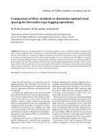
4. right skewed (S~0.8) with equal variances (transformation: 1/(0.5+x) with (0,1) uniform x).
5. exponential distribution (parameter λ=0.4) with μ=2.5 which is extremely skewed (S=2).
6. exponential distribution (parameter λ=0.4) with μ=2.5 rounded to integer values 1,2,..


Methodology of the study

9

7. lognormal distribution (parameters μ=0 and σ=0.25) which is slightly skewed (S=0.778)
and nearly resembles a normal distribution.
8. uniform distribution in the interval (0,5).
9. uniform distribution with integer values 1,2,...,5.
(First uniformly distributed values in the interval (0,5) are generated, then effects are added
and finally rounded up to integers.)
10. left and right skewed (transformation log2(1+x) with (0,1) uniform x).
(For two levels of B the values had been mirrored at the mean.)
11. left skewed (transformation log2(1+x) with (0,1) uniform x) with unequal variances on B
with a ratio max(si2)/min(si2) of 4.
12. left skewed (transformation log2(1+x) with (0,1) uniform x) with unequal variances on both
factors with a ratio max(si2)/min(si2) of 4.
13. normal distribution ( N(0,1) ) with unequal variances on both factors with a ratio
max(si2)/min(si2) of 3 for unequal cell counts where small ni correspond to small variances
(ni proportional to si) .

14. normal distribution ( N(0,1) ) with unequal variances on both factors with a ratio
max(si2)/min(si2) of 3 for unequal cell counts where small ni correspond to large variances.
(ni disproportional to si)
15. left skewed (transformation log2(1+x) with (0,1) uniform x) with unequal variances on both
factors with a ratio max(si2)/min(si2) of 3 for unequal cell counts where small ni correspond
to small variances (ni proportional to si).
16. left skewed (transformation log2(1+x) with (0,1) uniform x) with unequal variances on both
factors with a ratio max(si2)/min(si2) of 3 for unequal cell counts where small ni correspond
to large variances (ni disproportional to si).
log2 (1 + x)

0.8
0.4

0.6

Density

1.0
0.0

0.0

0.2

0.5

Density

1.0

1.5

1.2

1.4

1 / (0 .5 + x )

0.6

0.8

1.0

1.2

1.4

1.6

1.8

2.0

0.0

0.2

0.4

0.6

0.8

1.0

Figure 1: histograms of a strongly right skewed distribution (left) and
a left skewed distribution (right)
In the cases of heteroscedasticity the cells with larger variances do not depend on the design.
Subsequently i,j refer to the indices of factors A respectively B.
• For both designs and unequal variances on B the cells with j=1 have a variance ratio of 4 and
those with j=2 a ratio of 2.25.


Methodology of the study

10

• For both designs and unequal variances on A and B the cells with i=1 and j ≤ 2 have a variance ratio of 4 and those with i=2 and j ≤ 2 a ratio of 2.25.
(The values of the corresponding cells had been multiplied by 2 and 1.5 respectively.)
Concerning the uniform distribution originally only the version with integer values had been
part of the plot. Preliminary tests showed that there are sometimes large differences between the
results obtained with continuous uniform distributions and those obtained with values rounded
to integers. So the conclusion was to include both versions of uniform distributions into this study. As a consequence the exponential distribution has been considered once in the standard form
with continuous values, and once with values rounded to integers, mainly in the range of 1 to
18. These differences demanded for further inverstigations. The impact of discrete dependent
variables on the type I error rate has been studied in detail by Luepsen (2016a).
By the way, there are only few studies considering discrete distributions in their simulations.
One of them is by Mansouri et al. (2004) in which they studied the ART-procedure for continuous as well as for discrete variables. He found no remarkable differences in the performance.

But it has to be mentioned that they studied only designs with ni up to 10.
The main simulation study consists of three parts:
• The type I error rates are studied for a fixed ni (depending on the design) and fixed effect
sizes. For this purpose every situation had been repeated 5000 times. This seems to be the
current standard.
• Further the error rates are computed also for ni varying from 5 to 50 in steps of 5 and for fixed
effect sizes, in order to see on one side, if acceptable rates stay acceptable, and on the other
side, if too large rates get smaller with larger samples. For the same situations the power rates
are computed.
• Additionally the error rates are computed for increasing effect sizes, but fixed ni (depending
on the design), to see the impact of other nonnull effects within a model. The effect sizes are
varying from 0.1*s to 1.5*s in steps of 0.2*s (s being the standard deviation of the dv). For
the same situations the power rates are computed, but with effect sizes varying from 0.2*s to
0.9*s in steps of 0.1*s .
In contrast to the first part a repetition of 2000 times had been chosen for the computation of the
error rates and power for large ni as well as increasing effect sizes, not only because of the larger
amount of required computing time, but also because the main focus had been laid more in the
relation between the methods than in exact values. A preliminary comparison of the results for
the computation of the power showed that the differences between 2000 and 5000 repetitions
are negligible. By means of a unique starting value for the random number generator the results
for all situations rely on the same sequence of random numbers and therefore on identical samples. This should make the results better comparable.
There are several ways to look at the power of one effect:
• while varying the cell count ni, e.g. from 5 to 50 in steps of 5,
• while varying the effect size (of any effect), e.g. from 0.2*s to 0.9*s in steps of 0.1*s ,
• while varying the situation (distribution) for a fixed method.
The first two views (varying the cell counts and varying the effect size) should lead to similar
results. And it does, at least qualitative, though there are quantitative differences. The third view
reveals if there are methods superior to others in special situations. But as nearly all nonparametric methods performed best for right skewed distributions this view has not been persued.

Methodology of the study

11

Concerning the graphical representation of the power two graphs have been chosen:
• the absolute power as the proportion of rejections in percent and
• the relative power, which is computed as the absolute power divided by the 25% trimmed
mean of the power of the 8 methods for each n=5,...,50 or d=0.2*s,...,0.9*s.
The purpose of the relative power is to make differences visible in the area of small n or d where
the graphs of the absolute power of the 8 methods lie very close together.

4. 2

Effect sizes

The main focus had been laid upon the control of the type I error rates for α=0.05 and α=0.01
for the various methods and situations as well as on a comparison of the power for the methods.
For the computation of the random variates level/cell means had to be added corresponding to
the desired effect sizes. These are denoted by ai and bj for the level means of A and B corresponding to effects αi and βj , and abij for the cell means concerning the interaction corresponding to effects αi + βj + αβij .
For the subsequent specification of the effect sizes the following abbreviations are used (s being
the standard deviation):
• A(d):
a1=d*s, a2=0 for a 2*4 plan,
respectively a1= a2= d*s, a3= a4= 0 for a 4*5 plan
• B(d):
b1= b2= d*s, b3= b4= 0 for a 2*4 plan,
respectively b1= b2= d*s, b3= b4= b5= 0 for a 4*5 plan
• AB(d):
ab11= ab12= ab23= ab24= d*s , ab21= ab22= ab13= ab14= 0 for a 2*4 plan,
respectively ab11= ab12= ab21= ab22= ab34= ab35= ab44= ab45= d*s ,

ab31= ab32= ab41= ab42= ab14= ab15= ab24= ab25= 0 and ab13= ab23= ab33= ab43= d*s/2
for a 4*5 plan
In case of effects the uniform distribution has been transformed that x+d*s lies still in the interval (0,5).
The error rates had been checked for the following effect models:
• main effects and interaction effect for the case of no effects (null model, equal means),
• main effects and interaction effect for the case of one significant main effect A(0.6)
i.e. a weak impact of significant main effects,
• main effect for the case of a significant interaction AB(0.6)
i.e. a weak impact of significant interaction effect,
• main effect for the case of a significant main and interaction effect A(0.6) and AB(0.6)
i.e. a weak impact of significant effects.
• interaction effect for the case of both significant main effects A(0.8) and B(0.8)
i.e. a strong impact of significant main effects.
These are 7 models which are analysed for both a balanced and an unbalanced design. So there
are all in all 14 models.
For the power analysis of main effect A and the interaction AB the effect sizes had to be reduced


Methodology of the study

12

in order to distinguish better the power for cell counts between 20 and 50. The following situations and effect sizes had been chosen:
• power of main effect A(0.3) in case of no other effects,
• power of main effect A(0.3) in case of a significant effect B(0.3),
i.e. impact of other significant main effects,
• power of main effect A(0.3) in case of a significant interaction AB(0.4),
i.e. impact of other significant effects,
• power of main effect A(0.3) in case of a full model (B(0.3) and AB(0.4))
i.e. impact of other significant effects,

• power of interaction effect AB(0.4) for the case no main effects,
• power of interaction effect AB(0.4) for the case of a significant main effect A(0.3),
i.e. impact of another significant main effect,
• power of interaction effect AB(0.4) in case of a full model (B(0.3) and B(0.3))
i.e. impact of other effects.

4. 3

Handling right skewed distributions

Concerning right skewed distributions preliminary tests revealed that all nonparametric methods under consideration here show increasing type I error rates with an increasing degree of heteroscedasticity which is due to the ranking.
Rather unproblematic behaves the exponential distribution because it has only one parameter
for both mean and variance. So there is no differentiating between the cases of equal and
unequal variances. To analyze the influence of effects d it is not reasonable to add a constant
d*s to the values x of one group. In order to keep the exponential distribution type for the alternative hypothesis (H1) a parameter λ‘ had to be chosen so that the desired mean difference
1/λ − 1/λ‘ is d*s where in this case s=(1/λ + 1/λ‘). As a consequence the H1-distribution has
not only a larger mean but also a larger variance.
In contrast the lognormal distribution reveals a more unfriendly behavior: all nonparametric
methods under consideration here show increasing type I error rates for increasing sample sizes
in the case of heterogeneous variances. A more precise investigation of the error rates of the
lognormal distribution has been done recently by Luepsen (2016b), who confirmed earlier results by Carletti & Claustriaux (2005) and Zimmerman (1998). Tables of the type I error rates
for the tests of the null model for all methods and various situations are to be found in appendix
A 6. As the behavior does not differ essentially for different parameters, a lognormal distribution with parameters μ=0 and σ2=0.25 has been chosen for the comparisons here. Its shape resembles slightly the normal distribution with a long tail on the right. As distribution for the
alternative hypothesis (H1) a shift of the distribution of the null hypothesis (as described in the
previous section) is one choice, thus keeping equal variances. But with real life right skewed
data the distribution of the alternative hypothesis often includes a change both of means and variances. In this case a different lognormal distribution had to be selected for H1 so that the means
have the desired difference, e.g. x and x +d*s, but slightly different variances. Preliminary tests
for the calculation of the power showed that both models produce nearly the same results.
Therefore the first method has been preferred because of the easier computational handling.
Additionally another right skewed distribution (above number 4) is included that has a form

comparable to the lognormal distribution with parameters μ=0 and σ=0.8, but restricted to the


Results

13

interval [0.67 , 2], or also comparable to a right shifted exponential distribution. This approaches real data sometimes better because the long tails on the right side are rare in practice. Here
the same method for constructing the distribution for the alternative hypothesis is used: a simple
shift to the right according to the desired effect size, whereas in the case of the exponential
distribution a different distribution with parameter λ‘ is chosen as H1-distribution which keeps
the same range of values but has a larger mean and larger variance. The user must decide which
model fits the data better.

5.
5. 1

Results
Tables and Graphical Illustrations

It is evident that a study considering so many different situations (8 methods, 16 distributions,
2 layouts, and 7 models) produces a large amount of information. Therefore the following
remarks represent only a small extract and will concentrate on essential and surprising results.
All tables and corresponding graphical illustrations are available online (see address below).
These are structured as follows, where each table and graphic includes the results for all 8
methods and report the proportions of rejections of the corresponding null hypothesis:
• appendix 1: type I error rates for α=0.05, α=0.01 and for fixed n, equal and unequal cell
counts,
• appendix 2: type I error rates for large n (5 to 50 in steps of 5) for α=0.05 and fixed effect
sizes, for equal and unequal cell counts and for different models,

• appendix 3: power in relation to n (5 to 50 in steps of 5) referring to α=0.05 and fixed effect
sizes, for equal and unequal cell counts and for different models,
• appendix 4: type I error rates for large effect sizes (0.1*s to 1.5*s in steps of 0.2*s ) for
α=0.05 and fixed n, for equal and unequal cell counts and for different models,
• appendix 5: power in relation to increasing effect sizes from 0.2*s to 0.9*s in steps of 0.1*s
for α=0.05 and fixed n, for equal and unequal cell counts and for different models,
• appendix 6: type I error rates for large n (5 to 50 in steps of 5) for α=0.05 and fixed effect
sizes for various lognormal distributions,
• appendix 7: type I error rates for small and large n (5, 10 and 50) for α=0.05 and fixed effect
sizes of the exponential and the uniform distributions, each for the version of a continuous
and three versions of a discrete distribution.
All references to these tables and graphics will be referred as A n.n.n. The most important tables
of A 1 and some graphics of A 2 to A 5 are included in this text.
All tables and graphics can be viewed online:
/>
5. 2

Type I error rates

A deviation of 10 percent (α + 0.1α) - that is 5.50 percent for α=0.05 - can be regarded as a
stringent definition of robustness whereas 25 percent (α + 0.25α) - that is 6.25 percent for
α=0.05 - to be treated as a moderate robustness (see Peterson, 2002). It should be mentioned
that there are other studies in which a deviation of 50 percent, i.e. (α −
+ 0.5α), Bradleys liberal
criterion (see Bradley, 1978), is regarded as robustness. As a large amount of the results concerns the error rates for 10 sample sizes ni = 5,...,50 it seems reasonable to allow a couple of


Results

14

exceedances within this range.
(In this chapter the values in brackets will refer to the error rates.)
Performance for small n
Let us first have a look onto the results for fixed ni = 5 and ni =10 (appendix A 1) and start with
the parametric F-test at the 5 percent level. All the well known results could be confirmed: on
one side departures from the normal distribution can be neglected, even in the case of a strongly
skewed distribution, but on the other side heterogeneous variances will lead to an inflation of
the type I error rate (6.00), especially in the case of unequal cell counts (over 8.00) or skewed
distributions (between 6.00 and 9.00) (see table 3 as well as tables 1-1-1 and 1-2-1 in A 1). For
the case of unequal ni Feir & Toothaker (1974) as well as Weihua Fan (2006) reported that the
F-test tends to be conservative if cells with larger ni have also larger variances and that it reacts
liberal if cells with larger ni have the smaller variances. This phenomenon is here confirmed
(table 8 as well as table 1-2-2 in A 1) and shows that the error rate may rise over 20 (at a nominal
5 percent level) for a variance ratio of 3 and a cell count ratio of 4.
Concerning the other methods there are also no spectacular results. In the null model (tables 3
and 5 as well as tables 1-1-1 and 1-2-1 in A 1) the ART and ART+INT show only decent exceedances of the moderate robustness in the case of unequal variances. Here applying the INT
to the ART shows a dampening effect as already remarked by Carletti & Claustriaux (2005).
Additionally there are a few large error rates for the INT- and one for the v.d.Waerden-test also
in the case of heterogeneous variances with values between 6 and 7 and once 8.4. The RT can
always hold the level, and the Puri & Sen- as well as the ATS-procedures even stay in the interval of stringent robustness. And in the challenging case of an unbalanced design where small ni
are paired with large si only the ATS keeps the error level under control, whereas in the case
where small ni are paired with small si of course all tests show acceptable rates (table 8 as well
as table 1-2-2 in A 1). So far this confirms the results mentioned in chapter 3.
When there is a nonnull main effect (table 6 as well as tables 1-3-1 and 1-4-1 in A 1 for balanced
designs and table 7 as well as table 1-4-3 in A 1 for unbalanced designs) again only the ART
and ART+INT exceed the interval of moderate robustness where also here the ART+INT has
the lower values. The INT-procedure has only for unbalanced designs slightly increased values,
mainly in cases of variance heterogeneity. And finally when both main effects are significant
(tables 1-3-2 and 1-4-2 in A 1) again the rates of the ART and ART+INT for the interaction

effect exceed the interval of moderate robustness in the cases of unequal variances. But here
also the RT shows too large error rates in the same situation. Table 6 and 7 demonstrate on one
side the increase of the error rates for the RT and the ATS if there are nonnull effects in the case
of unequal variances, while on the other side the rates for the Puri & Sen and the v.d.Waerden
decrease generally as stated before.
Similar results were obtained at the 1 percent level though results at that level tend to be more
liberal in general. Figure 2 shows the distribution of the error rates for the interaction for the
different situations. For an easier identification heteroscedastic distributions are marked red,
right skewed distributions green and uniform distributions blue.
But for increasing sample sizes ni things look quite different at least in some settings.


Results

15

.

0
unequal
no effects

2

4

6

8 10 12

unequal
A sig

unequal
A and B sig
ATS
P&S
vd Waerden
ARTINT
ART
INT
RT
param

equal
no effects

equal
A sig

equal
A and B sig

ATS
P&S
vd Waerden

normal
norm B hetero
norm A B hetero

right skew ed
expo cont
expo discr
lognormal
unif cont
unif discr
r/l skew ed
skew ed A hetero
skew ed A B hetero

ARTINT
ART
INT
RT
param
0

2

4

6

8 10 12

0

2

4

6

8 10 12

observed type I error rate

Figure 2: type I error rates for the interaction at the 5 percent level for all distributions
considered, equal and unequal cell counts, three models and for various distribution types
Performance for large n: right skewed distributions
Right skewed distributions occur in practice rather frequently, and often their shape, e.g. that of
the lognormal distribution, is not much different from that of a normal distribution. But this
difference causes an inflation of the type I error rate in conjunction with unequal variances.
Most of them are only visible for larger samples. This effect had been reported by Zimmerman
(2004) generally for skewed distributions, and for the lognormal distribution by Carletti &
Claustriaux (2005) as well as recently by Luepsen (2016b), especially if the ART-method is
applied.
In case of the lognormal distribution - as mentioned in chapter 4 - the error rates of the tests of
the null model rise generally for all nonparametric procedures with increasing ni above the
acceptable limit. The extent differs from the distribution parameters, especially from the
skewness and from the degree of variance heterogeneity. As here variances are assumed as
equal these effects are not reflected in this study. Only for the test of a main effect, if the other


Results

16

is significant, the error rate for the ART-method in an unbalanced design is not controlled (see
A 2.4.7). For larger skewed lognormal distributions, e.g. with parameters μ=0 and σ2=1, things

look a bit different: As remarked by Luepsen (2016b) the ART- and to a less degree also the
ART+INT-technique cannot keep the type I error under control even for homogeneous variances and equal cell counts, with rates usually between 8 and 11 percent. The detailed results
are tabulated in A 6.
For the exponential distribution it has to be remarked that in all situations the type I error rates
of the ART-procedure rise beyond the acceptable limit for ni larger than 10 or 20 (see e.g.
A 2.3.5, 2.4.5, 2.6.5 and 2.8.5 with values between 9 and 20), except for the tests of the null
model. And the ART performs even worse in the version with integer values. This phenomenon
had been analyzed in detail and explained by Luepsen (2016a). As a consequence the same
applies also to the ART+INT-procedure, but to a less degree: only for the test of main effects in
unbalanced designs the a level is offended. Additionally there are a couple of situations where
the RT reacts liberal: for the test of a main or interaction effect if both other effects are nonnull.
The other right skewed distribution (marked as no 4 in chapter 4) acts comparatively gently.
Only for the test of a main effect in unbalanced designs if there are other nonnull effects the rates
of the ART+INT, and to a less degree of the ART, rise beyond the acceptable limit (see e.g. A
2.4.4, 2.6.4 and 2.8.4 with values between 9 and 28 for the ART+INT, and values between 6
and 18 for the ART). One reason for this different behavior is the different method for constructing the distribution for the alternative hypothesis (see section 4.3).
Performance for large n: other distributions
Concerning the parametric F-test there are no deviations from the above described behavior
obvious for large ni . And table 1 confirms the robustness of the parametric test in regard to
unequal variances as long as the sample sizes are equal. Perhaps to mention: Exceeding error
rates decrease often with increasing ni (see e.g. A 2.2.12, A 2.4.3 and A 2.6.12) which had to be
expected from the central limit theorem.
Elsewise the nonparametric procedures. Looking at the basic tables for ni=5 and ni=10 their
behavior appears mostly in the acceptable area. But for larger ni some show rising error rates,
especially the ART, ART+INT, RT, ATS and sometimes the INT and the Puri & Sen procedures. The following peculiarities do neither concern those unbalanced designs where ni are correlated with si nor discrete distributions that will be looked at later.
Generally the ART tends to be liberal with rates above the acceptable limit of moderate robustness (beyond 6) in the cases of heterogeneous variances (see e.g. figure 3). Additionally there
is the situation of the test for a main effect (for which the ART is not primarily designed) in an
unbalanced design, if there are other nonnull effects (see figure 4 as well as A 2.4, 2.6 and 2.8).
Here the error rates rise to 10 and above when ni (ni > 15) increases up to 50.
The ART+INT shows a similar performance as the ART which is plausible from the procedure.

But mostly its rates lie below those of the ART as remarked by Carletti & Claustriaux (2005).
Additionally there are several settings of heterogeneous variances where the ART+INT keeps
the error rate completely under control: e.g. all tests of main effects (see figure 4 and A 2.1 and
A 2.2). And finally one additional positive aspect: In the case where unequal cell frequencies
are paired with unequal variances the ART+INT is the only method (beside the ATS) that keeps
the error rate under control, at least for the test of main effects (see e.g. table A 1-2-2 for small
ni as well as sections 11 and 13 in A 2.2, A 2.4, A 2.6 and A 2.8).


Results

17

Also for the RT the error rates lie beyond the limit in the situations of unequal variances. But
these are fewer here. It occurs for the tests for main and interaction effects when there is another
nonnull effect, with values increasing up to 10 and sometimes above when ni (ni > 15) increases
up to 50 (see figure 3 and see sections 2 and 3 as well as 11 an 12 in A 2.3 to A 2.8 and A 2.11
to A 2.14). But it has to be remarked that they stay in the acceptable region for ni < 15. This is
the phenomenon described in section 2.1, but happening here only in the case of unequal variances. Finally it should be remarked that the RT has lower rates than the ART in all noticeable
cases except the last mentioned designs with nonnull main effects.
The Puri & Sen- and the ATS-method show both the same behavior as the RT-procedure. While
the ATS has nearly the same error rates, those of the Puri & Sen-method lie clearly lower,
especially if there are other nonnull effects. This conservative behavior was explained in section
2.5. So the Puri & Sen-method keeps the type I error rate often in the moderate robustness interval, frequently even the stringent robustness interval at least for small and moderate ni <25,
in situations where the RT exceeds the limits (see e.g. A 2.6.3, 2.7.3, 2.7.11, 2.11.12 or 2.13.2).
If the Puri & Sen-method offends the criterion then only for larger ni (ni ≥ 30). As for the RT:
the ATS is only acceptable for small ni < 15.
effect
(model)

des param

A

eq

(null model)

ne

B

eq

(A sig)
A
(AB sig)
B
(A+AB sig)
AB
(null model)
AB
(A sig)
AB
(A+B sig)

ne

RT

3C

3C

eq

INT

C

B

AC

ART

ART+
INT

4689BC

69

6

69

56BC

A

1...6 8...C 1...6 8...C

Puri & van der
Sen Waerden

ATS

C

B

B

23BC

23569BC

69

23BC

23BC

ne 3 5 6 C

23B

1....C

1....C

2B

2B

eq

356

45

56BC

A

56

56

356C

2456C

1....C

1....C

356C

56

BC

236BC

2C
C

C

ne

3C

eq

2B

ne

3BC

C

3BC

eq

B

23BC

2

2356BC

2C

ne

3C

24B

34C

369BC

39C

eq

B

ne

2356BC 23456C

2369BC 369BC

56BC

3BC 23456BC 3456BC 2369BC

39C

23B

356C

23BC
2B

3C

2356BC

C

2356BC

Table 1: Violations of the type I error rates in the range of ni = 5,...,50
The numbers refer to the distibutions (see chapter 4.), A to right/left-skewed distributions, B and
C to left skewed distributions with unequal variances. The layout has the following meaning:
n: moderate - values outside the interval of moderate robustness, but mostly below 7
n: strong - nearly all values above 7
n: rising - values inside the interval of moderate robustness for ni < 15, but rising for larger ni
„eq“ and „ne“ in the column „des“ refer to equal and unequal cell counts.

Results

18

The INT-procedure has of course also some problems with unequal variances but predominantly in unbalanced designs showing slightly increased error rates between 7 and 10 (see e.g. A
2.4.11, 2.10.12 and 2.13.12). Additionally the rates rise above the limit in a couple of cases with
underlying skewed distributions and equal variances (see A 2.4.10, 2.7.4, 2.8.4 and A 2.14.4).
And finally the behavior seems to be generally slightly liberal for the test of the interaction if
both other effects are nonnull (see A 2.13 and A 2.14).
The van der Waerden-test is the less conspicuous from all methods. The shape of the graph of
its rates looks much alike them of the INT-method, which is not surprising considering the
computation, but the values lie clearly lower. So there exist only three instances where the
error rate is unsatisfactory: the test of main or interaction effects in the unbalanced null model
in the case of skewed distributions with unequal variances on both factors (values between 6
and 7, see A 2.2.12 and 2.10.12), and the test of a main effect in a full model with an underlying exponential distribution.
Special situations
It remains to look at unbalanced designs where ni are correlated with si . Concerning the type I
error rate, the case when small ni correspond to small si is unproblematic. Here nearly all methods keep the error level under control. Only when there are other nonnull effects, the ART- as
well as the ART+INT-technique reveal increasing rates as already mentioned above (see
A 2.4.13 and A 2.4.15). Here the performance of the ART is acceptable for ni < 20 and of the
ART+INT for ni < 30.
In the challenging case where small ni correspond to large si the ATS-method is the only one
that keeps the error level under control for all models. Nevertheless it should be remarked that
the the Puri & Sen-procedure shows acceptable rates for the test of the main and interaction
effect if the other effects are nonnull (see A 2.14.14 and A 2.14.16). But this has to be regarded
as exceptions.
Discrete Variables
Though all the nonparametric procedures under consideration here, except the ATS, require a
continuous dependent variable, in practice they are applied to discrete variables as well and

often even to ordinal variables with only a few distinct values.
Comparing all 8 methods with regard to the behavior in the case of underlying discrete distributions, exponential and uniform, the tables and graphics in appendix 2 show that the type I error
rates rise mainly for the ART- and the ART+INT-procedures for increasing cell counts ni, in
most cases beyond 10 percent, but sometimes even up to 20 percent. See e.g. A 2.5.6, 2.5.9,
2.10.6, 2.10.9, situations where the rates remain in the interval of moderate robustness for the
corresponding continuous distribution. But in any case the error rates for the discrete distribution lie considerably above those for the continuous distribution, on average between 10 and
more than 100 percent. For details see summary tables A 7.15.3 (exponential distribution) and
A 7.15.4 (uniform distribution).
In the case of the uniform distribution the situation is more transparent because for the continuous distribution the error rates the ART- and the ART+INT-procedures are always under
control, except one case: the test of a main effect if the other main effect is nonnull. For the discrete distribution the rates stay below 6 percent for all other models as long as n i ≤ 15 and rise
up to values between 6 and 8 if ni increases up to 50. But it has to be noted that at least for equal
cell counts the rates keep acceptable for most models, especially for the test of the interaction,


Results

19

though they lie between 10 and 20 percent above those for the continuous distribution. See the
table in A 7.15.4 for details which represents a summary of the results for the ART-method
tabulated in A 2.
On the contrary all other methods behave mostly in the normal range. Only for the test of the
interaction in the case of significant main effects the values for the RT, INT and ATS (between
8 and 10) lie beyond the acceptable limit for large ni (see A 2.13.6 and 2.14.6).
A detailed study about the impact of discrete dependent variables comes from Luepsen (2016a)
in which also an explanation of this phenomenon is given. Additionally it is shown that the error
rates rise beyond the interval of moderate robustness if the number of distinct values decreases,
and this more severe for the exponential than for the uniform distribution.
Summary
The results for the parametric F-test confirm its „classical“ behavior: the test controls the type

I error as long as either the sample sizes or the variances are equal. Nonnormal distributions
have nearly no impact.
The ART- and the ART+INT-procedures have deficiencies with heterogeneous variances, with
discrete variables, with (even slightly) right skewed distributions and with the test of main
effects in unbalanced designs. This makes these methods not recommendable. And the positive
results mentioned in chapter 4 are not valid in general.
The RT-, ATS- and Puri & Sen-method have generally problems with unequal variances, even
for balanced designs. And these problems enlarge for tests in those cases when there are other
nonnull effects. On the other side the ATS is the only method that can handle in all situations
the challenging case of unbalanced designs with unequal variances where small ni correspond
to large si. But also for the ATS it must be admitted that the control of the type I error rate cited
in chapter 3 is no more valid for larger samples.
The INT-method is in many cases acceptable though there are a number of unsatisfying situations for which there is no guideline visible.
From this it is obvious that the van der Waerden-test has the fewest violations. Table 1 gives an
impression of the distribution of error rates offending the limits for the different situations.

5. 3

Power

In this study only the relation between the power of the different nonparametric anova methods
is examined whereas the absolute power values that are achieved are of minor interest. The results for equal and unequal cell counts are only conditionally comparable because of the different number of cells as well as the different cell counts.
From the previous section it is obvious that, besides the van der Waerden-test, the nonparametric methods are scarcely able to achieve amelioration for the cases of unequal cell frequencies paired with unequal variances compared with the parametric F-test. Therefore the
focus is laid here on those settings with non-normal distributions where nonparametric methods
are supposed to reach a higher power than the parametric F-test. Of course there are situations
in which tests react liberal, leading on one side to high power rates, but also on the other side to
offending the type I error rate. Such situations will be neglected here.


Results

20

Performance of the different methods
At first the power for the various methods shall be discussed. As a general result, considering
all forms of distribution and effect situations, it can be concluded that the methods based on the
inverse normal transformation (INT, ART+INT and v.d. Waerden) show constantly a high power, and in most cases even the best power (see figure 5), perhaps except in the case of exponential distributions. The ART+INT performs best when there are also other effects present.
Sometimes the superiority of the ART+INT method starts only with ni > 10 (e.g. for factor A in
the case of unequal cell counts, see A 3.2). The INT and v.d. Waerden methods are the best for
the power of main effect A in the case of unequal cell counts. But as to be expected (see remarks
in section 2.6) the power of the v.d.Waerden test worsens, compared to others, if there are other
significant effects (see figure 5 and table 2 as well as A 3.7, A 3.8, A 3.13 and A 3.14). And this
applies in a boosted degree to the interaction effect. There are no essential differences, neither
between the balanced and the unbalanced design nor between the power of factor A and the
power of the interaction AB.
The ART-procedure shows high power rates in all cases of underlying normal distributions with
heterogeneous variances, though it weakens for the special case if both main effects are significant, but not the interaction. It is also a good choice for the exponential distribution as well
as for left skewed distributions with heterogeneous variances, but in both cases only for small
ni ≤ 15. But unfortunately these are the situations where the ART shows a liberal reaction for
the type I error. In all other cases, especially in the cases of an underlying uniform distribution,
the ART is no good choice because its power is rather poor.
There are only a few situations where the RT method performs satisfactorily: in cases of underlying normal distributions with unequal variances if there are no other effects present. And the
performance worsens when there are also other effects and is rather poor for the full model. Also
for the RT holds: the good performance occurs in those situations where the error rates exceed
the limits.
And the ATS and Puri & Sen methods which keep the type I error rate the best in many cases?
In general these are among those with the lowest power. Table 2 demonstrates that these have
never an above-average power. Both have frequently the lowest power, e.g. for the interaction
effect (see e.g. A 3.11 and 3.13) and for the main effect in the full model (see e.g. A 3.7 and
3.8). The Puri & Sen procedure is the worst for the main and interaction effects in the full model

when there are also significant main effects (see e.g. A 3.7 and 3.11). The latter effect is plausible because the reduction of error sum of squares induced by significant main effects cannot
be exploited by the Puri & Sen method. This applies also to the van der Waerden method but in
that case this negative effect is compensated by the normal transformation. The ATS is the worst
performer for the interaction effect in unbalanced designs with power rates about 40 percent
below average (see e.g. A 3.10 and 3.12). Nevertheless there are a few situations in which the
ATS excels positively: in unbalanced designs with heterogeneous variances if large ni correspond to large si (see A 3.2.13, 3.2.15, 3.10.13, 3.10.15, 3.14.13 and 3.14.15).
And what about the power of the parametric F-test? In general its power lies in the middle of
the results, except for a few situations: In the ideal case of an underlying normal distribution
with homogeneous variances the F-test is of course the best performer though the lead to the
nonparametric methods is negligible. In models with more than one significant effect, e.g. the
full model, the F-test is able to score (see table 2). And finally for unbalanced designs with heterogeneous variances if small ni correspond to large si, the parametric test is among the best
(see e.g. A 3.2.14, 3.2.16, 3.4.14, 3.4.16, 3.12.14, 3.12.16 and 3.14.14). A special comment is


Results

21

necessary for the right skewed distributions. On one side the parametric F-test is the absolute
winner for the much skewed exponential distributions. On the other side for the right skewed
distribution (no 4) the power of the F-test is the lowest of all: up to 40 percent (for the interaction
if there are no other effects) below the best performing INT and v.d.Waerden procedures (see
e.g. A 3.8.4 or 3.14.4). Table 2 also demonstrates that for this type and for uniform distributions
(4, 5 and 6) the F-test is always inferior to the INT-based methods. One explanation is the different method for choosing the H1-distribution (see section 4.3).
effect
des
(side effects)

param

A

eq

56

(none)

ne

56

A

eq

56

(B sig)

ne

56

A

eq

2356ABC

(AB sig)

ne 1 2 3 5 6 A B C

A

eq

RT

ART

ART+
INT

Puri van der
ATS
Sen Waerden

4789AB

23C

489AB

489AB

2

8A

489AC

23C56

3489ABC

489A

9

489AC

249 14789ABC
4789AB
24 134789ABC

2356BAC

(B+AB sig) ne 1 2 3 5 6 A B C

INT

47

489ABC

2356BC

2 3 4 8...C

4 8 9...C

456789ABC

2356BC

1 2 3 4 8...C

489AB

489AB

2356BC

2...4 5 6 7 8...C

89B

1 4 7 8..A B C

123456BC

1 2 3 4...C

89B

4689AB

2356C

489AB

489A

46789ABC

2356B

1489ABC

489A

AB

eq

56

(none)

ne

356

AB

eq

12356BC

456789ABC

2356BC

23489ABC

4 6 8 9..C

(A sig)

ne

1 2 3 5 6 9...C

1 2 3 4...A B C

2356BC

1 2 3 4 5 7 8..C

4 5.. B

AB

eq 1 2 3 5 6 A B C

1...5 6...B C

2 3 4 5 6 B C 1 2...4 5 6 7...C

6 8.. B

(A+B sig)

ne 1 2 3 5 6 A B C 1 4 7

1 2 3 4...B C

2

2 3 4 5 6 7 B C 1 2...4 7 8...C

6 8.. C

Table 2: Above-average power performance in the range of ni = 5,...,50
The numbers refer to the distributions (see chapter 4), A (10) to right/left-skewed distributions,
B (11) and C (12) to left skewed distributions with unequal variances. The layout has the following meaning:
n: moderate - power at least 5 percent above the average
n: moderate - power at least 5 percent above the average, only for large samples (above ni > 20)
n: moderate - power at least 5 percent above the average, only for small samples (below ni < 20)
n: strong - power at least 10 percent above the average
„eq“ and „ne“ in the column „des“ refer to equal and unequal cell counts.

Table 2 gives an impression of the distribution of above-average power performances. For every
sample size a performance value - in the graphics of appendix A 3 denoted by relative power is computed as the percentage of power above the mean over the 8 methods, which is computed
as a 25% trimmed mean. These values are averaged over all sample sizes ni = 5,...,50 as well as
for small sizes ni = 5,...,20 and for large sizes ni = 25,...,50. This table demonstrates among
others the poor performance of the Puri & Sen- and the ATS-methods which never show values
that lie 5 percent above the average. Further it shows that the power of the v.d.Waerden-test

Results

22

shrinks when there are side effects and of course the good performance of the INT- and
especially of the ART+INT-procedure.
Performance for non-normal distributions
For underlying exponential distributions, both in the continuous and in the discrete version, the
parametric F-test is without restrictions the best performer. In most instances the ART-technique is able to keep up for small sample sizes ni ≤ 15, but worsens for larger ni . But: the ART
violates the type I error control in these cases. For unbalanced designs the INT- and the
v.d.Waerden-procedures are often also a good choice.
For the lognormal distribution the differences between the power rates of the different methods
are generally rather small. But in most situations the INT- and the v.d.Waerden-procedures are
the leader, followed by the ART+INT-technique.
The case of an underlying right skewed distribution (marked as no 4 in chapter 4) is eye-catching insofar as the differences are the largest of all situations: in general up to 40 percent between the smallest and the largest power (see e.g. A 3.1.4 and 3.14.4). The best methods here are
the INT- and the v.d.Waerden-procedure though the ART+INT-method can keep up as long as
not all effects are significant.
For the uniform distributions, both in the continuous and in the discrete version, the methods
based on the inverse normal transformation (INT, ART+INT and v.d. Waerden) show constantly the best power. And the differences between these are minimal. For discrete uniform distributions the ART+INT is often the leader. But that cannot be utilized because of its bad type I error
behavior. The parametric F-test lies generally below the INT-based methods in the medium
range, while all other procedures show comparatively low power rates and reach often only 60
to 70 percent of the top values (see e.g. A 3.10.8 and 3.14.8).
Also for the case of mixed left/right-skewed distributions the INT-based methods have the
highest power rates, followed by the parametric F-test. Concerning the INT- and the ART+INTprocedures this result is only useful for the test of interaction effects because they failed to
control the type I error for the tests of a main effect.
Again for left skewed distributions with heterogeneous variances the INT-based methods are
among the best performers. Here the parametric F-test and the ART-technique can in fact also
score, but their type I error behavior is insufficient in these cases. Unfortunately the INT- as well

as the ART+INT-method show also increased error rates for this kind of distributions, at least
for unbalanced designs. So the only recommendable procedure left is the van der Waerden-test.
It remains to remark that the differences between the power rates are generally small.
Special situations
Now a glance shall be put on some of the situations concerning the distributions and effect
combinations.
In the case of a full model the ART+INT-method yields generally high power rates, both for the
main and the interaction effects. But: for the main effect in unbalanced designs its error rates
are not under control.
In the various cases of underlying normal distributions the differences between the methods are
rather small as long as there are no influences by other effects. In the case of a full model, i.e.
all effects being significant, the differences rise up to about 30 percent (see e.g. A 3.8.2, 3.8.3


Results

23

as well as 3.13.3 and 3.14.3).
Of special interest will be the case of unequal variances because, as stated in the previous section, nearly all methods suffer from unacceptable type I error rates in such instances. First the
case of an underlying normal distribution. The only methods not strongly affected by the heteroscedasticity are the Puri & Sen- and the v.d.Waerden-tests which differ only little from the
computational view, the ART+INT-technique except for the test of interaction effects in
unbalanced designs, and the parametric F-test for balanced designs. The overall performance of
the v.d.Waerden-method is slightly better than that of the Puri & Sen-method (see. e.g. A 3.5.3
and 3.8.2), though in the case of the null model the power of the latter lies about 2 percent higher
(see e.g. A 3.2.3 and 3.10.2). However the ART+INT in general as well as the parametric F-test
for the cases of equal sample sizes reach often higher power rates than the other two methods,
especially in models with nonnull side effects, e.g. the full model (see table 2 as well as e.g.
A 3.7.2 and A 3.7.3). Second the case of non-normal distributions. Here was indicated in the
previous section that the v.d.Waerden-test is to prefer.

Finally the case of unequal cell counts together with unequal variances. If small ni correspond
to small si the ATS is the best performer (see e.g. A 3.2.13 and A 3.2.15). If this method is not
implemented the ART as well as the RT method can be applied. If small ni correspond to large
si the high values of the parametric F-test and the INT-method are not helpful because of their
poor type I error control. Therefore the v.d.Waerden-procedure is the only suitable one showing
good results (see e.g. A 3.2.14 and A 3.2.16), especially in the case of an underlying skewed
distribution.
Summary
Summarizing the results so far: The van der Waerden-method is generally among the good performers, though it weakens for small ni if there are also other nonnull effects. Just in these situations of a full model the ART+INT-procedure is recommendable, especially for underlying
normal distributions with unequal variances and for lognormal distributions. The INT-method
is a good choice for all right skewed and uniform distributions as long as there are no heterogeneous variances. The ART reveals a good performance just in those cases where its type I error behavior is unsatisfactory. And finally the parametric F-test reaches a high power for the
exponential distribution, and of course for normal distributions, but in the case of unequal variances only for balanced designs.
When later an overall good performing method is looked for, considering all results, it might be
helpful to know which are the worst performers concerning the power. Often there are only
small differences, but there are some situations in which the power of the tests differ strongly,
for example in the full models and for the tests of the interaction in general. In these cases the
Puri & Sen-, the RT- and the ATS-method are definitely the losers (see table 2 and A 3.7 to
A 3.14). Beside this the ART is among the worst for the tests of the interaction (see e.g. A 3.9
and A 3.10) and the tests of the main effect when the other main effect is nonnull (see A 3.4).
Also the van der Waerden method shows a vulnerable point: unbalanced designs when small ni
are paired with small si , but only in the case of an underlying normal distribution. And finally
the parametric F-test is sometimes the worst: in unbalanced designs when small ni are paired
with small si .


Results

5. 4

24

Impact of effect size on the Type I error rates

At first sight the overall decreasing error rates of the Puri & Sen and the van der Waerden
methods for rising effect sizes are remarkable (see e.g. A 4.1.1 and 4.6.1). But this is easy to
explain: As mentioned in section 2 both tests are based on χ2 ratios with MStotal , the total mean
square of the total variation, in the denominator. And with increasing effect sizes of other effects
in the model this denominator is getting larger and making the ratio of the considered effect and
therefore also the χ2 ratio smaller.
Completely unacceptable are the error rates of the ART (up to 30 for values of 1.5*s) for growing effect sizes in the cases of an underlying exponential distribution (see e.g. A 4.1.5, 4.2.5,
4.3.5, 4.4.6 etc). The same applies to the ART and the ART+INT for the test of the main effects
in unbalanced designs if there are also other nonnull effects in the model. Their error rates rise
up to 10 percent and beyond for values of 1.5*s of the side effects (see A 4.2 and A 4.4). These
phenomena correspond to those described for large n in the previous section.
It remains to have a look on the performance of the RT since it is said to show increasing error
rates for the interaction if there are also significant main effects (see section 2.1). There is only
a slight increase to observe with maximum rates between 7 and 10 percent for effect sizes of
1.5*s in the cases of heterogeneous variances (see sections 2 and 3 as well as 8 and 9 in A 4.5
and A 4.7) and in the case of the exponential distribution (see A 4.7.5), both in balanced designs.
And as stated by Huang (2007) the INT keeps the error rate under control in these situations.
But an exception is to be observed: for nonnormal distributions with unequal variances in
unbalanced designs (see sections 8 and 9 in A 4.6 and A 4.8). By the way a similar behavior of
the RT is to be observed for the test of the main effects in a balanced design (see sections 2 and
3 as well as 8 and 9 in A 4.3).
Finally it has to remarked that the ATS-method performs rather similar to the RT-method. All
other methods behave inconspicuously.

5. 5

Impact of effect size on the Power

The impact of the effect size on the power is more of theoretical than of practical interest. For,
the researcher knows normally little of the real sizes of the effects in the model, but he knows
the cell counts, and sometimes he is even able to influence the ni. In general the results for varying effect sizes are similar to those for varying cell counts.
First it must be remarked that the power for all tests (main and interaction effects) in unbalanced
models is lower than in balanced designs, though the smaller ni is counterbalanced by the larger
number of cells. And this applies particularly to the tests in the full model.
The ART-technique shows a power above mean, at least for smaller ni ≤ 15, in the cases of heteroscedacity, but unfortunately here this method often cannot control the type I error rate. In
contrast, the performance of the ART in the case of the uniform distribution proves to be rather
poor and is often the worst (see e.g. A 5.1.8 and 5.4.8). Here the ART+INT performs considerably better. A look at the results for main and interaction effects in full models shows that the
ART+INT is a good choice for balanced designs whereas the INT is preferable for unbalanced
designs. Finally: because of the liberal attitude of the ART for the exponential distribution, as
stated in the previous section, its high power rates in that case are neither surprising nor helpful.
The same results apply to the ART+INT-technique, though it is not always superior to the ART.
Whereas the van der Waerden-method showed generally a good performance concerning the