An empirical study of the risk-free rate and the expected consumption growth

Journal of Applied Finance & Banking, vol. 9, no. 6, 2019, 67-90
ISSN: 1792-6580 (print version), 1792-6599(online)
Scientific Press International Limited

An empirical study of the risk-free rate and the
expected consumption growth
Weiwei Liu 1

Abstract
This paper studies the relationship between the risk-free rate and the expected
consumption growth. Using the monthly time series data from 2002.01-2017.12,
we obtain the following empirical evidences: 1) In the whole period, US supports
the positive intertemporal substitution effect and rejects the negative precautionary
saving effect. Accordingly, China rejects the positive intertemporal substitution
effect and supports the negative precautionary saving effect. 2) In the subsample
period 2002.01-2008.12, US and China generate the consistent results and both
support the CRRA asset pricing model. 3) The estimated time discount factors are
0.9995 and 0.9966 for US and China respectively. 4) US has a relative risk
aversion than China both in the whole sample and subsample.
JEL classification numbers: G12, E21
Keywords: Risk-free rate; Consumption growth; Asset pricing; Intertemporal
substitution; Precautionary saving

1. Introduction
The risk-free rate is an important factor in macroeconomics and finance. When
people worry about the uncertainty of the economy or the future, the precautionary
saving demand will rise. This will lead to the increase of the investment growth
and the decrease of the consumption growth, and therefore result in the
descending of the risk-free rate. The economic intuition is obvious that the
risk-free rate comoves with the consumption growth in the same direction. From
the perspective of consumption-based asset pricing theory, the relationship

between them seems to be positive and linear. The purpose of this paper is to
1

PBC School of Finance, Tsinghua University, Beijing 100083, China.

Article Info: Received: June 2, 2019. Revised: June 19, 2019
Published online: September 10, 2019


68

Weiwei Liu

verify the effectiveness of the theory using the empirical time series data of US
and China. Scholars have found some affecting factors of the risk-free rate, such
as the GDP growth rate, the unemployment rate, the inflation rate, the capital
marketization, the stock market return and volatility, the monetary policy and so
on. We implement a detailed literature survey in section 2 and treat some of these
factors as the control variable in our empirical setting of section 4.
In general, we need to consider three aspects of factors which are the economic
fundamentals, the monetary policy and the capital market. In China, the interest
rate liberalization is an important reform policy of the economy and now it is still
under way. In the prophase and metaphase stage, the interest rate is expected to go
up. In addition, within the economic transformation period the dependence of the
investment, the real estate, and the land will dramatically decline. Then the
demand of the capital will rise which will cause a high interest rate. We use the
one-year government bond rate as the proxy of risk-free rate in the long run and
use the inter-bank offered rate (IBOR) or the benchmark deposit rate as the proxy
in the short run. Due to the rigid payment problem in China, using the three-month
government bond rate will underestimate the risk-free rate after year 2010.

Therefore, after 2010 some studies use the wealth-management products rate as
the proxy. In US, there is a high degree of capitalization and the interest rate is
market-oriented so there are less fluctuations and misestimations in the US
risk-free rate. We use one-year government bond rate as the proxy of risk-free rate
in the long run and three-month treasury bill rate in the short run.
We take the expected aggregate consumption growth of the whole economy as the
independent variable. To estimate the expected consumption growth of this month,
we apply last month’s consumption growth as the substitute or the average of the
last N months consumption growth as the alternative options (N could be 3, 6 or
12). The detail will be discussed it section 4 which is the empirical analysis
section.
The software SAS is used for programming and implementing all the regressions.
The basic empirical method or technique is the time series analysis and the
sensitivity analysis. The method of instrumental variable is supposed to be used
for solving the omitted variable problem or reciprocal causation problem.
The remaining of this article is organized as follows. Section 2 contains the
literature review and the innovation of this paper. Section 3 displays the
theoretical framework and the assumptions. Section 4 describes the data and
presents the empirical results. Section 5 concentrates on the robustness check with
subsample analysis. Section 6 concludes.


An empirical study of the risk-free rate and the expected consumption growth.

69

2. Literature review
2.1 Related theory and literature
Risk-free rate has been discussed in plenty of top journals such as JF, JFE, RSF,
JFQA etc. These studies mainly focus on the risk-free rate puzzle that the CCAPM

fails to interpret the low risk-free rate in US and on the term structure of interest
rates. As for the study of consumption, the household consumption risk and the
risk aversion are the hottest topics. There is a gap between the asset pricing theory
and the empirical evidence from different countries. This paper tries to directly
link the
risk-free rate with the consumption growth under the controlling of other
important variables. Some related papers are summarized as follows.
Lin and Jen (1980) constructed the theoretical model which linked the
consumption, the investment, the market price and the risk-free rate all together.
The model was a new version of CAPM, which showed that the risk-free rate is
not an exogenous variable and, therefore, must be determined jointly with other
endogenous variables. It is a good attempt to explain the risk-free rate and the
consumption growth. Because of the lack of data in that period, the empirical
evidence was hard to be provided. Lettau and Ludvigson (2001) used the quarterly
data of consumption, wealth and found that the fluctuations in the
consumption-wealth ratio are strong predictors of excess stock return over a
Treasure bill rate. Since the return of risk asset can be predicted by the
information of consumption, the risk-free rate should not be excluded in the
prediction process. We follow their research and define the consumption as the
nondurable goods and service including food and clothes. And we update the data
to 2017. Constantinides and Ghosh (2017) showed that shocks to consumption
growth are negatively skewed, persistent, countercyclical, and drive asset prices.
There are also some studies focusing on the impact of the consumption on house
prices, through some channels such as wealth effect (Carroll et al., 2011),
mortgage effect (Compbell and Cocco, 2007), substitution effect (Sheiner, 1995)
and so on. Whether these effects are existing in risk-free assets is an important
research question for further studies.
The literature studying the main influence factors of the risk-free rate are as
follows. Watcher (2006) developed a consumption-based model of the term
structure of interest rate and discovered that nominal bonds depends on past

consumption growth and on expected inflation. Chien and Lustig (2010)
introduced limited liability in a model with a continuum of ex ante identical agents
that face aggregate and idiosyncratic income risk and found the negative
correlation between risk-free rate and the expected excess stock return and
positive correlation with the Pstor-Stambaugh liquidity. Chen (2017) decomposed
the risk-free rate in intertemporal substitution effect (−𝐸𝑡 (𝑚𝑡+1 )) and the
1
precautionary saving effect (− 2 𝑉𝑎𝑟𝑡 (𝑚𝑡+1 )). They found that the intertemporal
substitution effect increased sharply in the bad times while the precautionary


70

Weiwei Liu

saving effect was much too small to smooth the risk-free rate.
The literature above contains mainly the research of the top finance journals which
focus on the US stock market. There are also some Chinese studies concentrated
on this topic but using the Chinese data to implement the empirical analysis. Wang
(2002) analyzed Chinese consumption, risk-free rate and the stock index and
showed that there are negative relations between stock index revenue rate and
consumption growth rate while under the condition of non-marketization of
interest rate in China, the changes of interest rate is not connected to consumption.
Jing (2007) analyzed the risk-free rate and the time preference (β) theoretically. In
their view, risk-free rate is the compensation for time preference, while risk return
is the compensation for people's risk aversion characteristics. Li, Wang and Yang
(2009)
studied the Chinese risk-free rate and the households’ consumption growth using
the Chinese monthly data from 1998-2008. However, their sample was too small
since they actually used the annual historical mean to estimate the asset pricing

model and obtained a negative coefficient of relative risk aversion. Deng (2014)
studied the asset pricing model with habit formation and empirically found that the
risk-free rate of China from 1995-2011 was highly related to the consumption
growth and volatility, the stock market return and volatility. These studies pointed
out the important problem of the interest rate marketization reform in China.
Empirical researches are still necessary to be carried forward in this field.
2.2 The contribution of this paper
This paper has four key contributions to the existing studies. Firstly, we fill the
gap between classic consumption-based asset pricing theory and the empirical
evidence on the relationship of risk-free rate and the consumption growth.
Secondly, we use the historical mean of consumption growth to approximate the
expected consumption growth and check the effectiveness of different expectation
periods. Thirdly, we test the hypothesis and estimate the relative risk aversion
coefficient and the time discount factor. This finding will provide some support on
the CRRA utility function theory. Finally, we compare the US results with the
Chinese results and find the inconsistence of the two countries in the whole
sample and the consistence in the subsample. These findings may bring up some
policy suggestions on the reform of China’s interest rate liberalization.

3. Theoretical framework
According to the consumption-based asset pricing model (Cochrane 2005), an
investor always targets at maximizing his total utility of today and the future as
follows.
U(𝑐𝑡 , 𝑐𝑡+1 ) = u(𝑐𝑡 ) + β𝐸𝑡 [u(𝑐𝑡+1 )]

(1)


An empirical study of the risk-free rate and the expected consumption growth.

71

Many scholars of asset pricing assume that the utility function takes the CRRA
form for convenience.
1

u(𝑐𝑡 ) = 1−𝛾 𝑐𝑡 1−𝛾

(2)

Where 𝛾 is the coefficient of the relative risk aversion.
If the investor tries to maximize the total utility of the investor at time 𝑡 given the
endowment 𝑒𝑡 , he faces the following conditions.
max U(𝑐𝑡 , 𝑐𝑡+1 ) = u(𝑐𝑡 ) + β𝐸𝑡 [u(𝑐𝑡+1 )] 𝑠. 𝑡.
𝑞

𝑐𝑡 = 𝑒𝑡 − 𝑝𝑡 𝑞
{𝑐
𝑡+1 = 𝑒𝑡+1 + 𝑥𝑡+1 𝑞

(3)

Where 𝑝𝑡 is the asset price at time 𝑡, 𝑥𝑡+1 is the sum of the asset price 𝑝𝑡+1
and the dividend 𝑑𝑡+1 . The asset can be stocks, bonds, derivatives and so on. 𝑞
is the
quantity of the asset, we assume that the endowment is divided either into
consumption or into investment.
We solve the first order condition and get the basic asset pricing condition which
is
𝑝𝑡 = 𝐸𝑡 [β

Where 𝑚𝑡+1 = β

u′ (𝑐𝑡+1 )
u′ (𝑐𝑡 )

= β𝑐

𝑐𝑡 𝛾

𝑡+1

𝛾

u′ (𝑐𝑡+1 )
𝑥𝑡+1 ]
u′ (𝑐𝑡 )

(4)

is the stochastic discount factor or the pricing

kernel. By definition, the return of the asset is given by
𝑅𝑡+1 =

𝑝𝑡+1 +𝑑𝑡+1
𝑝𝑡

=

𝑥𝑡+1

𝑝𝑡

= 𝑟𝑡+1 + 1

(5)

So, we can rewrite the equation (4) as following form
𝐸𝑡 [𝑚𝑡+1 𝑅𝑡+1 ] = 1

(6)

Since the asset can be anything, we consider the risk-free asset and assume the
risk-free rate is relatively stable as the time goes. We must have
𝑓

𝐸𝑡 [𝑚𝑡+1 𝑅𝑡+1 ] = 1
1

𝑓

𝑅𝑡+1 = 𝐸 [𝑚
𝑡

𝑡+1 ]

=

(7)
1

𝑐 𝛾
𝐸𝑡 [β 𝑡 𝛾 ]
𝑐𝑡+1

(8)


72

Weiwei Liu
1

We assume that β = 𝑒 𝛿, where 𝛿 is a positive parameter and close to zero, so β
is close to 1. Then equation (8) can be wrote as
𝑓

𝑅𝑡+1 =

Where Δ𝑙𝑛𝑐𝑡+1 = ln(

1
𝑐 𝛾
𝐸𝑡 [β 𝑡 𝛾 ]
𝑐𝑡+1

𝑐𝑡+1
𝑐𝑡

=

1
𝑐 𝛾
ln( 𝑡 𝛾 )
𝐸𝑡 [𝑒 𝛿 𝑒 𝑐𝑡+1 ]

= {𝐸𝑡 [𝑒 −𝛿−𝛾Δ𝑙𝑛𝑐𝑡+1 ]}−1

(9)

) is the consumption growth and we additionally

assume that it obeys the normal distribution.
Δ𝑙𝑛𝑐𝑡+1 ~𝑁𝑜𝑟𝑚𝑎𝑙(𝜇, 𝜎 2 )

(10)

Let z = −𝛿 − 𝛾Δ𝑙𝑛𝑐𝑡+1, then z also obeys the normal distribution. According to
the two formulas in econometrics, we know that
1 2
(𝑧)

{

E(𝑒 𝑧 ) = 𝑒 𝐸(𝑧)+2𝜎
Var(𝑒 𝑧 ) = 𝑒 2𝐸(𝑧)+𝜎

2 (𝑧)(𝑒 𝜎2 (𝑧) −1)

(11)

Therefore equation (9) changes to
𝑓

𝑅𝑡+1 = 𝑒 𝛿+𝛾𝐸𝑡

1
2

(Δ𝑙𝑛𝑐𝑡+1 )− 𝛾2 𝜎𝑡2 (Δ𝑙𝑛𝑐𝑡+1 )

(12)

𝑓

Since 𝑅𝑡+1 is the gross risk-free rate, then the risk-free rate is
𝒇

𝒇

𝒇

𝒓𝒕+𝟏 = 𝐥𝐧(𝑹𝒕+𝟏 ) ≈ 𝑹𝒕+𝟏 − 𝟏

(13)

Combining equation (12) and (13), we obtain the relationship between risk-free
rate and expected consumption growth described by equation (14)
𝒇

𝒇

𝟏

𝒓𝒕+𝟏 = 𝐥𝐧(𝑹𝒕+𝟏 ) = 𝜹 + 𝜸𝑬𝒕 (𝚫𝒍𝒏𝒄𝒕+𝟏 ) − 𝟐 𝜸𝟐 𝝈𝟐𝒕 (𝚫𝒍𝒏𝒄𝒕+𝟏 )

(14)

By now we have displayed the theoretical foundation of the relationship between
risk-free rate and consumption growth. All those are based on five assumptions:
1) The CRRA utility function hypothesis of the representative investor.
2) The normal distribution of the consumption growth.
3) The endowment is divided either into consumption or the investment (no
trading cost).
1
4) The time discount factor β has the form as β = 𝑒 𝛿 and close to 1.
5) The stock market is efficient and investors are rational.


An empirical study of the risk-free rate and the expected consumption growth.

73

Equation (14) is the crucial theoretical foundation we try to verify. This CRRA
model is just a benchmark asset pricing model since there are more complicated
models such as the Campbell and Cochrane model, the Epstein and Zin model et
al. In next section, we will describe the data and the empirical model setting. Then
we will test the assumptions and discuss the empirical results.

4. Empirical analysis
4.1 Data sources

This article collects the US data from the WIND database and Amit Goyal’s
website ( while the
Chinese data is all from WIND database. All these data are monthly time series
from 2002.01 to 2017.12 (192 months in total). The consumption data is the total
sales of the nondurable goods and service for each month. We implement the
seasonal adjustments. The US risk-free rate is three-month treasure bill rate while
the Chinese risk-free rate is the one-year government bond return according to
study on Chinese risk-free rate. Since Chinese data frequency of government bond
return is daily, we use average of daily returns of one month as the risk-free rate
and transform the annual rate to monthly rate. The S&P500 index and the
Shanghai Composite Index are used to calculate the monthly stock return and
volatility for US and China respectively.
4.2 Variables description
4.2.1 Overview of the variables
𝑓
The explained variable is the risk-free rate 𝑅𝑡+1 , the explanatory variables are the
expected consumption growth and the variance of the consumption growth, the
control variables are the inflation rate, the expected return of stock market and the
volatility of the stock return. We use 3 months, 6 months and 12 months historical
mean of the consumption growth to estimate the expected consumption growth
and apply the same method to the expected stock return. The most convenient way
is to use last month’s consumption growth as an approximate of the expected
consumption growth. We will discuss it in the next subsection. Since the GDP is
the endowment of the whole economy and consumption which already contains
some information of GDP is directly related to the risk-free rate, so the GDP
growth is not included in the control variables for this paper.
The expected consumption growth and the expected return of stock market and the
corresponding variances take the following form.
1

𝐸𝑡 (Δ𝑙𝑛𝑐𝑡+1 ) = 𝑇 ∑𝑇𝑖=1 Δ𝑙𝑛𝑐𝑡+1−𝑖
𝟏

𝑬𝒕 (𝑹𝒕+𝟏 ) = 𝑻 ∑𝑻𝒊=𝟏 𝑹𝒕+𝟏−𝒊

(15)
(16)


74

Weiwei Liu

𝟏

𝝈𝟐𝒕 (𝚫𝒍𝒏𝒄𝒕+𝟏 ) = 𝑻 ∑𝑻𝒊=𝟏( 𝚫𝒍𝒏𝒄𝒕+𝟏−𝒊 − 𝑬𝒕 (𝚫𝒍𝒏𝒄𝒕+𝟏 ))𝟐
𝟏

𝝈𝟐𝒕 (𝑹𝒕+𝟏 ) = 𝑻 ∑𝑻𝒊=𝟏( 𝚫𝒍𝒏𝑹𝒕+𝟏−𝒊 − 𝑬𝒕 (𝑹𝒕+𝟏 ))𝟐

(17)
(18)

Τ can be 1, 3, 6, 12 for different length of the expectation of the agent. Table 1
displays the description of the variables.
Table 1: Description of all the variables

Variable label
Rfree
Cg

E_Cg1
E_Cg3
E_Cg6
E_Cg12
V_Cg3
V_Cg6
V_Cg12
Rt
E_Rt1
E_Rt3
E_Rt6
E_ Rt 12
V_ Rt 3
V_ Rt 6
V_ Rt 12
infl

Variable expression
𝑓
𝑅𝑡+1

Δ𝑙𝑛𝑐𝑡+1
𝐸𝑡 (Δ𝑙𝑛𝑐𝑡+1 ) T=1
𝐸𝑡 (Δ𝑙𝑛𝑐𝑡+1 ) T=3
𝐸𝑡 (Δ𝑙𝑛𝑐𝑡+1 ) T=6
𝐸𝑡 (Δ𝑙𝑛𝑐𝑡+1 ) T=12
𝜎𝑡2 (Δ𝑙𝑛𝑐𝑡+1 ) T=3
𝜎𝑡2 (Δ𝑙𝑛𝑐𝑡+1 ) T=6
𝜎𝑡2 (Δ𝑙𝑛𝑐𝑡+1 ) T=12
𝑅𝑡+1

𝐸𝑡 (𝑅𝑡+1 ) T=1
𝐸𝑡 (𝑅𝑡+1 ) T=3
𝐸𝑡 (𝑅𝑡+1 ) T=6
𝐸𝑡 (𝑅𝑡+1 ) T=12
𝜎𝑡2 (𝑅𝑡+1 ) T=3
𝜎𝑡2 (𝑅𝑡+1 T=6
𝜎𝑡2 (𝑅𝑡+1 ) T=12

inflation

Explanation
Risk-free rate
Consumption growth
Expected consumption growth T=1
Expected consumption growth T=3
Expected consumption growth T=6
Expected consumption growth T=12
Variance of consumption growth T=3
Variance of consumption growth T=6
Variance of consumption growth T=12
Stock return
Expected stock return T=1
Expected stock return T=3
Expected stock return T=6
Expected stock return T=12
Variance of stock return T=3
Variance of stock return T=6
Variance of stock return T=12
Inflation rate

4.2.2 The descriptive statistics
The descriptive statistics of all the variables are shown in Table 2.1 and Table 2.2
below. Table 2.1 displays the descriptive statistics of all the variables for US data,
while Table 2.2 displays the descriptive statistics of all the variables for Chines
data.


An empirical study of the risk-free rate and the expected consumption growth.

75

Table 2.1: Descriptive statistics of all the variables for US data

Variables
Rfree
Cg
E_Cg1
E_Cg3
E_Cg6
E_Cg12

Size
192
192
192
192
192
192

Mean

0.0010
0.0029
0.0028
0.0028
0.0028
0.0028

Std
0.0013
0.0092
0.0092
0.0058
0.0043
0.0033

Min
0.0000
-0.0374
-0.0374
-0.0326
-0.0210
-0.0102

Max
0.0042
0.0289
0.0289
0.0126
0.0092
0.0074

t-statistics
10.92
4.39
4.22
6.70
8.92
11.56

V_Cg3

192

0.0001

0.0001

0.0000

0.0016

6.34

V_Cg6

192

0.0001

0.0001

0.0000

0.0009

8.65

V_Cg12

192

0.0001

0.0001

0.0000

0.0005

11.62

Rt

192

0.0061

0.0409

-0.1832

0.1042

2.06

E_Rt1

192

0.0059

0.0409

-0.1832

0.1042

2.02

E_Rt3

192

0.0062

0.0256

-0.1172

0.0767

3.34

E_Rt6

192

0.0058

0.0200

-0.0903

0.0567

4.03

E_ Rt 12

192

0.0053

0.0145

-0.0473

0.0358

5.10

V_ Rt 3

192

0.0010

0.0015

0.0000

0.0091

9.36

V_ Rt 6

192

0.0013

0.0014

0.0000

0.0075

12.61

V_ Rt 12

192

0.0015

0.0015

0.0001

0.0075

14.60

infl

192

0.0017

0.0039

-0.0192

0.0122

6.13

Note: All the data are monthly time series from 2002.01-2017.12

As shown in Table 2.1, the average risk-free rate of one month is 0.10% with a

standard deviation of 0.13%. The average consumption growth rate is 0.29% with
a standard deviation of 0.92%. The average expected consumption growth rate is
0.28% with a standard deviation of 0.92%, 0.58%, 0.43%, 0.33% for the
expectation periods T=1, 3, 6, 12 respectively. A moving average of longer
horizon brings about smaller fluctuations for the expected consumption growth
rate. The mean return of the stock market S&P 500 index of one month is 0.61%
which means an annual return of 7.57%, and with a standard deviation of 4.09%.
The average monthly inflation rate is 0.17% implying an annual inflation rate of
2.06% which is consistent with the circumstances of US economy. And the
deviation is 0.39% monthly.


76

Weiwei Liu

Table 2.2: Descriptive statistics of all the variables for Chinese data
Variables
Size
Mean
Std
Min
Max
t-statistics
Rfree
192
0.0021
0.0006
0.0008
0.0034

48.65
Cg
192
0.0112
0.0575
-0.1536
0.1654
2.70
E_Cg1
192
0.0120
0.0585
-0.1536
0.1654
2.84
E_Cg3
192
0.0120
0.0322
-0.0861
0.0841
5.16
E_Cg6
192
0.0121
0.0195
-0.0407
0.0554
8.57
E_Cg12

192
0.0119
0.0034
0.0020
0.0233
49.13
V_Cg3

192

0.0024

0.0027

0.0000

0.0154

11.95

V_Cg6

192

0.0030

0.0021

0.0007

0.0092

20.28

V_Cg12

192

0.0034

0.0009

0.0019

0.0076

51.98

Rt

192

0.0036

0.0809

-0.2828

0.2425

0.62

E_Rt1

192

0.0033

0.0810

-0.2828

0.2425

0.57

E_Rt3

192

0.0034

0.0520

-0.1578

0.1410

0.91

E_Rt6

192

0.0030

0.0417

-0.1265

0.1229

1.00

E_ Rt 12

192

0.0026

0.0322

-0.1031

0.0980

1.12

V_ Rt 3

192

0.0038

0.0053

0.0000

0.0315

9.98

V_ Rt 6

192

0.0048

0.0048

0.0002

0.0190

14.10

V_ Rt 12

192

0.0056

0.0046

0.0005

0.0199

16.79

infl

192

0.0022

0.0060

-0.0130

0.0260

5.08

Note: All the data are monthly time series from 2002.01-2017.12

As shown in Table 2.2, China is much different with US in many variables. The
average risk-free rate of one month is 0.21% with a standard deviation of 0.06%.
China has higher risk-free rate with lower volatility than US. The average
consumption growth rate is 1.12% with a standard deviation of 5.75%. It is not

surprising that the consumption growth rate is three times higher than US because
of the high GDP growth rate in China (Over 7% each year). The average expected
consumption growth rate is 1.20% with a standard deviation of 5.85%, 3.22%,
1.95%, 0.34% for the expectation periods T=1, 3, 6, 12 respectively. A moving
average of longer horizon also brings about smaller fluctuations for the expected
consumption growth rate and it is more obvious than US. The mean return of the
stock market Shanghai composite index of one month is 0.36% which means an
annual return of 4.41%, and with a standard deviation of 8.09%. The risk of the
Chinese stock market is higher than US. The average monthly inflation rate is


An empirical study of the risk-free rate and the expected consumption growth.

77

0.22% implying an annual inflation rate of 2.67% which is consistent with the
circumstances of Chinese economy. And the deviation is 0.60% monthly.
4.3 Model set up
The empirical model is based on the theoretical framework of asset pricing in
section 3. Equation (14) is a benchmark relation between the risk-free rate and the
expected consumption growth with the CRRA utility function. The risk-free rate is
decomposed to two components which are intertemporal substitution effect and
precautionary saving effect. For more general utility functions such as Campbell
and Cochrane model and the Epstein and Zin model, the expected stock return
(risk assets) is also an influence factor of the risk-free rate. Since the purpose of
this paper is to provide some empirical evidences for the relationship between
risk-free rate and the expected consumption growth rate, we treat the expected
stock market return as one of the control variables. In addition, we take the
volatility of the stock return into consideration. By the reason of using nominal
variables (including risk-free rate and consumption growth rate), we also

incorporate the inflation rate (derived by CPI) into control variables. Then the
empirical model is set up as follow
𝑓

𝑟𝑡+1 = 𝛽0 + 𝛽1 𝐸𝑡 (Δ𝑙𝑛𝑐𝑡+1 ) + 𝛽2 𝜎𝑡2 (Δ𝑙𝑛𝑐𝑡+1 ) + 𝛾 ′ 𝑋𝑖𝑡 + 𝜀𝑡+1

(19)

Where 𝒓𝒇𝒕+𝟏 is the explained variable, 𝐸𝑡 (Δ𝑙𝑛𝑐𝑡+1 ) and 𝜎𝑡2 (Δ𝑙𝑛𝑐𝑡+1 ) are the
explanatory variables, 𝜷𝟏 and 𝜷𝟐 are two coefficients respectively. The 𝑿𝒊𝒕 is
the vector of control variables and 𝜸′ is the vector of the coefficients. Table 3
displays the variable categories.
Table 3: Variable categories

Variables
𝑓
𝑟𝑡+1

Variable categories
explained variable

Variables contained
Rfree

𝐸𝑡 (𝛥𝑙𝑛𝑐𝑡+1 ) explanatory variables

E_Cg1, E_Cg3, E_Cg6, E_Cg12

𝜎𝑡2 (𝛥𝑙𝑛𝑐𝑡+1 ) explanatory variables

V_Cg3, V_Cg6, V_Cg12

𝑋𝑖𝑡

control variables

E_Rt1, E_Rt3, E_Rt6, E_Rt12
V_Rt3, V_Rt6, V_Rt12, infl

4.4 Empirical results of US
The software SAS is used for the data cleaning, data arrangement and the
regression process. The data is monthly time series from 2002.01 to 2017.12. We
implement the regression with different expectation periods T=3, 6, 12. In general,
significance of the coefficients increases dramatically when the expectation period


78

Weiwei Liu

T goes up from 3 to 12. When T=1, the estimated coefficient is 0.0055 with a
t-statistics of 0.54 which is not significant. Different options of regressions with
control variables are included for comparison. The results are presented in Table
4.1, 4.2, 4.3 respectively.
Table 4.1: The regression on risk-free rate using US data when T=3

(1)
constant
E_Cg3

0.0010***
(9.37)
0.0169
(1.06)

V_Cg3

(2)
0.0009***
(8.20)
0.0174
(1.09)
0.7646
(1.09)

E_Rt3

(3)
0.0009***
(8.16)
0.0265
(1.36)
0.7590
(1.08)
-0.0036
(-0.82)

(4)

(5)

0.0009***
(7.52)
0.0100
(0.61)
0.7089
(1.02)

0.0009***
(7.45)
0.0210
(1.08)
0.6981
(1.00)
-0.0046
(-1.04)

0.0442*
(1.83)
192
0.0294

0.0471*
(1.94)
192
0.0350

V_Rt3
infl
N

𝑅2

192
0.0059

192
0.0121

192
0.0156

(6)
0.0011***
(7.83)
0.0070
(0.35)
0.7691
(1.13)
-0.0063
(-1.44)
-0.1956***
(-2.98)
0.0387
(1.62)
192
0.0541

Note: In parentheses is the t value, ***, **, and * represent significant levels at 1%, 5%, and 10%
respectively. Data is monthly time series from 2002.01 to 2017.12.

The results Table 4.1 indicate that the coefficients of E_Cg3 and V_Cg3 are all
positive. For example, in column (2) the coefficients are 0.0174 and 0.7696 while
the t-statistics are 1.09 and 1.09 respectively. In column (3) and (5), the effect of
E_Rt3 is negative which implies that the risk-free rate and the expected stock
return move in the opposite direction. In column (4) and (5), the variable infl is
significant in 10% level and moves in the same direction with risk-free rate which
is consistent with the economic intuition. In column (6), V_Rt3 is also significant
but it reduces the significance of explanatory variables by a large margin. Since it
is not included in the equation of CCAPM model, this result is consistent with the
model implication. The R2 is improved from 0.0059 to 0.0541 with the control
variables added gradually.


An empirical study of the risk-free rate and the expected consumption growth.

79

Table 4.2: The regression on risk-free rate using US data when T=6

(1)
constant
E_Cg6

0.0009***
(8.36)
0.0334
(1.56)

V_Cg6

(2)
0.0008***
(6.02)
0.0421*
(1.92)
1.1939*
(1.68)

E_Rt6

(3)
0.0008***
(5.89)
0.0687**
(2.29)
1.0834
(1.52)
-0.0084
(-1.30)

(4)

(5)

0.0007***
(5.61)
0.0364
(1.65)
1.0067
(1.50)

0.0007***
(5.41)
0.0673**
(2.26)
0.9215
(1.29)
-0.0100
(-1.54)

0.0411*
(1.74)
192
0.0427

0.0456*
(1.93)
192
0.0547

V_Rt6
infl
N
𝑅2

192
0.0126

192
0.0272

192
0.0359

(6)
0.0013*
(7.64)
0.0307
(1.06)
1.4241**
(2.10)
-0.0180***
(-2.85)
-0.3709***
(-5.03)
0.0454**
(2.04)
192
0.1679

Note: In parentheses is the t value, ***, **, and * represent significant levels at 1%, 5%, and 10%
respectively. Data is monthly time series from 2002.01 to 2017.12.

The results Table 4.2 indicate that the coefficients of E_Cg6 and V_Cg6 are still
all positive and significant in column (2), (3) and (5). For example, in column (2)
the coefficients are 0.0421 and 1.1939 while the t-statistics are 1.96 and 1.68
respectively. In column (3) and (5), the effect of E_Rt6 is negative which implies
that the risk-free rate and the expected stock return move in the opposite direction.
In column (4) and (5), the variable infl is also significant in 10% level and moves
in the same direction with risk-free rate which is consistent with the economic

intuition. In column (6), V_Rt6 is also significant but it reduces the significance of
explanatory variables by a large margin. For example, the t-statistics of E_Cg6
decreases from 2.26 to 1.06 in column (5) and (6). Since it is not included in the
equation of CCAPM model, this result is consistent with the model implication.
The R2 is improved from 0.0126 to 0.1679 with the control variables added
gradually.
Compared with the case T=3, when T goes up from 3 to 6 the coefficients are
significant now and the R2 increases from 0.0541 to 0.1679.


80

Weiwei Liu
Table 4.3: The regression on risk-free rate using US data when T=12

(1)
constant
E_Cg12

0.0008***
(6.78)
0.0744***
(2.70)

V_Cg12

(2)
0.0004***
(3.04)
0.1058***

(3.59)
2.3173***
(2.70)

E_Rt12

(3)
0.0005***
(3.14)
0.1405***
(3.59)
1.8675**
(2.03)
-0.0129
(-1.35)

(4)

(5)

0.0005***
(2.82)
0.0990***
(3.34)
2.2043**
(2.57)

0.0005***
(2.91)
0.1356***

(3.47)
1.7212*
(1.87)
-0.0137
(-1.43)

0.0369
(1.61)
192
0.0853

0.0386*
(1.68)
192
0.0953

V_Rt12
infl
N
𝑅2

192
0.0370

192
0.0727

192
0.0816

(6)
0.0016***
(7.74)
0.0189
(0.50)
3.4137***
(4.07)
-0.0262***
(-3.06)
-0.5938***
(-7.53)
0.0440**
(2.19)
192
0.3067

Note: In parentheses is the t value, ***, **, and * represent significant levels at 1%, 5%, and 10%
respectively. Data is monthly time series from 2002.01 to 2017.12.

The results Table 4.3 indicate that the coefficients of E_Cg12 and V_Cg12 are all
positive and significant at level of 1% in column (2), (3), (4), (5) and (6). For
example, in column (2) the coefficients are 0.1058 and 2.3173 while the t-statistics
are 3.59 and 2.70 respectively. In column (3) and (5), the effect of E_Rt12 is
negative which implies that the risk-free rate and the expected stock return move
in the opposite direction. In column (4) and (5), the variable infl is significant in
10% level and moves in the same direction with risk-free rate which is consistent
with the economic intuition. In column (6), V_Rt12 is also significant. However, it
reduces the significance of explanatory variables even sharply. For example, the
t-statistics of E_Cg6 decreases from 3.47 to 0.50 in column (5) and (6). Since it is
not included in the equation of CCAPM model, this result is consistent with the

model implication. The R2 is improved from 0.0370 to 0.3067 with the control
variables added step by step.
Compared with the case T=6, when T goes up from 6 to 12 the coefficients are
more significant now. The significant level changes from 5% to 1% while the R2
increases from 0.1679 to 0.3067.
Since the case of T=12 is the best result, we may make some analyses regarding
this result. Firstly, the CRRA model implies the intertemporal substitution effect is
positive while the precautionary saving effect is negative. However, our empirical
evidence supports the positive intertemporal substitution effect but rejects the
negative precautionary saving effect. The estimation of the two corresponding
coefficients are 0.1058 and 2.3173 both at 1% significant level. The estimation of


An empirical study of the risk-free rate and the expected consumption growth.

81

coefficient of relative risk aversion γ is 0.1058 in column (2) and 0.1405 in
column (3). It reveals that the risk aversion of US investors is relatively low. The
estimation of the time preference parameter (the constant) is 0.0004, which
implies the discount factor β = 𝑒1𝛿 = 0.9996, which is consistent with the economic
theory.
4.5 Empirical results of China
The process is the same with last subsection except the data is Chinese data. The
data is monthly time series from 2002.01 to 2017.12. Similarly, we implement the
regression with different expectation periods T=3, 6, 12. When T=1, the estimated
coefficient is 0.0004 with a t-statistics of 0.56 which is also not significant for
Chinese data. Different options of regressions with control variables are included
for comparison. The results are presented in table 5.1, 5.2, 5.3 respectively. In
general, significance of the coefficients increases dramatically when the

expectation period T goes up from 3 to 12.
Table 5.1: The regression on risk-free rate using Chinese data when T=3

(1)
constant
E_Cg3

0.0021***
(45.25)
0.0010
(0.77)

V_Cg3

(2)
0.0022***
(35.44)
0.0008
(0.55)
-0.0257
(-1.60)

E_Rt3

(3)
0.0022***
(35.74)
0.0006
(0.45)
-0.0233

(-1.46)
-0.0017**
(-1.98)

(4)

(5)

0.0022***
(34.46)
0.0003
(0.18)
-0.0249
(-1.55)

0.0022***
(34.76)
0.0000
(0.00)
-0.0222
(-1.39)
-0.0018***
(2.10)

0.0077
(0.99)
192
0.0216

0.0094

(1.22)
192
0.0441

V_Rt3
infl
N
𝑅2

192
0.0031

192
0.0165

192
0.0365

(6)
0.0022***
(32.35)
-0.0003
(-0.18)
-0.0211
(-1.33)
-0.0023***
(-2.63)
-0.0185**
(-2.21)
0.0115

(1.50)
192
0.0685

Note: In parentheses is the t value, ***, **, and * represent significant levels at 1%, 5%, and 10%
respectively. Data is monthly time series from 2002.01 to 2017.12.

The results Table 5.1 indicate that the coefficients of E_Cg3 and V_Cg3 are
positive and negative respectively but not significant. For example, in column (2)
the coefficients are 0.0008 and -0.0257 while the t-statistics are 0.55 and -1.60
respectively. In column (3) and (5), the effect of E_Rt3 is negative and significant
at 1% level which implies that the risk-free rate and the expected stock return
move


82

Weiwei Liu

in the opposite direction. In column (4) and (5), the variable infl is not significant
but still move in the same direction with risk-free rate which is consistent with the
economic intuition. In column (6), V_Rt3 is significant but it reduces the
significance of explanatory variables by a large margin. Since it is not included in
the equation of CCAPM model, this result is consistent with the model implication.
The R2 is improved from 0.0031 to 0.0685 with the control variables added
gradually.
Table 5.2: The regression on risk-free rate using Chinese data when T=6

(1)
constant

E_Cg6

0.0021***
(41.40)
-0.0007
(-0.31)

V_Cg6

(2)
0.0023***
(26.48)
-0.0023
(-1.02)
-0.0603***
(-2.80)

E_Rt6

(3)
0.0023***
(26.46)
-0.0025
(-1.08)
-0.0593***
(-2.74)
-0.0008
(-0.80)

(4)

(5)

0.0023***
(24.55)
-0.0026
(-1.12)
-0.0560**
(-2.46)

0.0023***
(24.47)
-0.0029
(-1.23)
-0.0536**
(-2.33)
-0.0010
(-0.92)

0.0046
(0.58)
192
0.0420

0.0060
(0.75)
192
0.0463

V_Rt6

infl
N
𝑅2

192
0.0005

192
0.0402

192
0.0435

(6)
0.0025***
(23.98)
-0.0028
(-1.24)
-0.0583***
(-2.61)
-0.0017
(-1.58)
-0.0316***
(-3.51)
0.0068
(0.87)
192
0.1056

Note: In parentheses is the t value, ***, **, and * represent significant levels at 1%, 5%, and 10%

respectively. Data is monthly time series from 2002.01 to 2017.12.

The results Table 5.2 indicate that the coefficients of E_Cg6 and V_Cg6 are both
negative in column (2) to (6) but only V_Cg6 is significant. For example, in
column (2) the coefficients are -0.0023 and -0.0603 while the t-statistics are -1.02
and -2.08 respectively. In column (3) and (5), the effect of E_Rt6 is negative
which implies that the risk-free rate and the expected stock return move in the
opposite direction. In column (4) and (5), the variable infl moves in the same
direction with risk-free rate which is consistent with the economic intuition. In
column (6), V_Rt6 is significant and it makes no difference on the significance of
explanatory variables The R2 is improved from 0.0005 to 0.1056 with the control
variables added gradually.
Compared with the case T=3, when T goes up from 3 to 6 one of the coefficients
is significant now and the R2 increases from 0.0685 to 0.1056.


An empirical study of the risk-free rate and the expected consumption growth.

83

Table 5.3: The regression on risk-free rate using Chinese data when T=12

(1)
constant
E_Cg12

0.0023***
(14.25)
-0.0144
(-1.11)

V_Cg12

(2)
0.0034***
(11.61)
-0.0439***
(-3.13)
-0.2341***
(-4.52)

E_Rt12

(3)
0.0034***
(11.57)
-0.0439***
(-3.16)
-0.2264***
(-4.40)
0.0026**
(1.99)

(4)

(5)

0.0035***
(11.68)
-0.0463***

(-3.29)
-0.2349***
(-4.55)

0.0034***
(11.61)
-0.0457***
(-3.26)
-0.2280***
(-4.43)
0.0022*
(1.67)

0.0107
(1.54)
192
0.1145

0.0078
(1.09)
192
0.1276

V_Rt12
infl
N
𝑅2

192
0.0064

192
0.1034

192
0.1220

(6)
0.0036***
(12.58)
-0.0327**
(-2.39)
-0.2473***
(-5.01)
0.0015
(1.16)
-0.0396***
(-4.40)
0.0060
(0.88)
192
0.2099

Note: In parentheses is the t value, ***, **, and * represent significant levels at 1%, 5%, and 10%
respectively. Data is monthly time series from 2002.01 to 2017.12.

The results Table 5.3 indicate that the coefficients of E_Cg12 and V_Cg12 are
both negative and significant at level of 1% in column (2), (3), (4), (5) and (6). For
example, in column (2) the coefficients are -0.0439 and -0.2341 while the
t-statistics are -3.13 and -4.52 respectively. In column (3) and (5), the effect of

E_Rt12 is now positive which implies that the risk-free rate and the expected stock
return move in the different direction. In column (4) and (5), the variable infl
moves in the same direction with risk-free rate which is consistent with the
economic intuition. In column (6), V_Rt12 is also significant. However, it reduces
the significance of explanatory variables a little bit. The R2 is improved from
0.0064 to 0.2099 with the control variables added step by step.
Compared with the case T=6, when T goes up from 6 to 12 both the coefficients
are significant now. The significant level changes from no significance and 5% to
1% while the R2 increases from 0.1056 to 0.2099.
Since the case of T=12 is the best result, we may make some analyses regarding
this result. Firstly, the CRRA model implies the intertemporal substitution effect is
positive while the precautionary saving effect is negative. However, our empirical
evidence rejects the positive intertemporal substitution effect but supports the
negative precautionary saving effect. The estimation of the two corresponding
coefficients are -0.0439 and -0.2341 both at 1% significant level. The estimation
of coefficient of relative risk aversion γ is -0.0439 in column (2) and (3). It
reveals that the risk aversion of Chinese investors is negative which means the risk
preference of the Chinese investors. The estimation of the time preference


84

Weiwei Liu

parameter (the constant) is 0.0034, which implies the discount factor 𝛃 = 𝒆𝟏𝜹 =
𝟎. 𝟗𝟗𝟔𝟔, which is consistent with the economic theory.
4.6 The comparison of US and China
In this sector, we put the results of US and China together in case of T=12 for
comparison. Since the volatility of stock market return is not suitable to be the
control variable both in theory and our empirical finding, we drop it and consider

only the expected stock return and the inflation rate in the regressions. The
comparison of US and China is showed at table 6.
Table 6: The comparison of US and China when T=12

US

constant
E_Cg12
V_Cg12

(1)
0.0004***
(3.04)
0.1058***
(3.59)
2.3173***
(2.70)

E_Rt12

China

(2)
0.0005***
(3.14)
0.1405***
(3.59)
1.8675**
(2.03)
-0.0129

(-1.35)

(3)
0.0005***
(2.91)
0.1356***
(3.47)
1.7212*
(1.87)
-0.0137
(-1.43)

192
0.0816

0.0386*
(1.68)
192
0.0953

(4)
0.0034***
(11.61)
-0.0439***
(-3.13)
-0.2341***
(-4.52)

(5)
0.0034***

(11.57)
-0.0439***
(-3.16)
-0.2264***
(-4.40)
0.0026**
(1.99)

(6)
0.0034***
(11.61)
-0.0457***
(-3.26)
-0.2280***
(-4.43)
0.0022*
(1.67)

192
0.1220

0.0078
(1.09)
192
0.1276

V_Rt12
infl
N
𝑅2

192
0.0727

192
0.1034

Note: In parentheses is the t value, ***, **, and * represent significant levels at 1%, 5%, and 10%
respectively. Data is monthly time series from 2002.01 to 2017.12.

From Table 6, we obtain some important results. Firstly, the two coefficients of
expected consumption growth and the variance of consumption growth represent
the intertemporal substitution effect and precautionary saving effect. In the theory
of CRRA model, the two coefficients are supposed to one positive and one
negative. But the empirical finding reveals that the two coefficients are both
positive in US and both negative in China. And the coefficients are both
significant at 1% level in US and China. US supports the positive intertemporal
substitution effect and rejects the negative precautionary saving effect. China
rejects the positive intertemporal


An empirical study of the risk-free rate and the expected consumption growth.

85

substitution effect and supports the negative precautionary saving effect.
Secondly, the estimation of the time preference parameter (the constant) is
consistent with the theory both in US and China. The average estimation of the
constant in US is 0.0005, implying the discount factor β = 𝑒1𝛿 = 0.9995 . The
average estimation of the constant in China is 0.0034, implying the discount factor

1
β = 𝛿 = 0.9966.
𝑒
Thirdly, the average estimation of the coefficient of expected consumption growth
is 0.1273 or -0.0445 for US and China respectively. It means that relative risk
aversion γ is 0.1273 or -0.0445 in US and China. US investor is risk averse but
with a low degree while Chinese investor is a little bit risk preferred.
Fourthly, the risk-free rate comoves with the expected stock return in the opposite
direction in US but the same direction in China. In addition, the risk-free rate
comoves with the inflation rate in the same direction both in US and in China.
Finally, the R2 increases from 0.0727 to 0.0953 in US and increases from 0.1034
to 0.1276 in China. It is nearly the same for the level of R2 in US and China which
is reasonable in the time series regressions.

5. Robustness check
In section 5, we perform the following robustness check with subsample analysis.
We regress the basic regression (19) on the two subsamples 2002.01-2008.12 and
2009.01-2017.12 with the case of T=12.
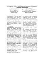
The reason of why we perform the subsample regression is that we find the rapid
decrease of the expected consumption growth rate in 2008 because of the 2008
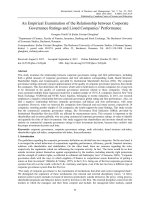
financial crisis. This phenomenon is more obvious in US. Figure 1.1 displays the
expected consumption growth in US and Figure 1.2 displays the expected
consumption growth in China.


86

Weiwei Liu

0,01

0,008
0,006
0,004
0,002
0
-0,002
-0,004
-0,006
-0,008
-0,01
-0,012

200201
200209
200305
200401
200409
200505
200601
200609
200705
200801
200809
200905
201001
201009
201105
201201
201209
201305

201401
201409
201505
201601
201609
201705

Expected consumption growth

Expected consumption growth in US

Time
Figure 1.1: The expected consumption growth in US

0,025
0,02
0,015
0,01
0,005

0
200201
200209
200305
200401
200409
200505
200601
200609
200705

200801
200809
200905
201001
201009
201105
201201
201209
201305
201401
201409
201505
201601
201609
201705

Expected consumption growth

Expected consumption growth in China

Time
Figure 1.2: The expected consumption growth in China

From figure 1 and 2, we can see that the expected consumption growth of China is
higher than US due to the rapid economic growth. What’s more, the expected
consumption growth decreases sharply in the year 2008, and reaches the bottom at
2008.12. To analyze this, we divide the sample into two samples which are
2002.01 to 2008.12 and 2009.01 to 2017.12. Table 7.1 shows the comparison of
US and China when T=12 before 2008.12. Table 7.2 shows the comparison of US
and China when T=12 after 2009.01

An empirical study of the risk-free rate and the expected consumption growth.

87

Table 7.1: The comparison of US and China when T=12 before 2008.12

US

constant
E_Cg12
V_Cg12

(1)
0.0018***
(6.82)
0.1508***
(2.72)
-1.6642*
(-1.70)

E_Rt12

(2)
0.0020***
(7.50)
0.0175
(0.24)
-0.3055

(-0.28)
0.0368**
(2.61)

China
(3)
0.0018***
(6.81)
0.1374**
(2.23)
-1.6824*
(-1.71)

(4)
0.0026***
(6.11)
0.0101
(0.52)
-0.1925***
(-3.36)

(5)
0.0024***
(5.34)
0.0169
(0.85)
-0.1620***
(-2.67)
0.0019
(1.44)

(6)
0.0026***
(6.14)
0.0080
(0.41)
-0.1937***
(-3.39)

V_Rt12
infl
N
𝑅2

84
0.1254

84
0.1940

0.0152
(0.51)
84
0.1281

84
0.2367

84
0.2561

0.0080
(1.15)
84
0.2491

Note: In parentheses is the t value, ***, **, and * represent significant levels at 1%, 5%, and 10%
respectively. Data is monthly time series from 2002.01 to 2008.12.

Table 7.1 shows that the coefficient of expected consumption growth is positive
while the coefficient of the variance of consumption growth is negative which is
consistent with the benchmark CRRA model. The results of China and US are
consistent for this subsample. The difference between them is that in US the
coefficient of the expected consumption growth is significant while in China the
coefficient of the variance of consumption growth is significant. For US result, the
average estimation of coefficient of relative risk aversion γ is 0.1018. The
average estimation of the time preference parameter (the constant) is 0.0019,
which implies the discount factor β = 𝑒1𝛿 = 0.9981, which is consistent with the
economic theory. The average R2 is 0.1492. For Chinese result, the average
estimation of coefficient of relative risk aversion γ is 0.0117. The average
estimation of the time preference parameter (the constant) is 0.0025, which
implies the discount factor β = 𝑒1𝛿 = 0.9975, which is consistent with the economic
theory. The average R2 is 0.2473.


88

Weiwei Liu

Table 7.2: The comparison of US and China when T=12 after 2009.01

US

constant
E_Cg12
V_Cg12

(1)
0.0002***
(4.25)
-0.0115
(-1.13)
-0.7471
(-1.59)

E_Rt12

(2)
0.0003***
(4.26)
-0.0188
(-1.19)
-0.8302*
(-1.69)
0.0018
(0.60)

China
(3)
0.0002***

(4.06)
-0.0115
(-1.02)
-0.7459
(-1.57)

(4)
0.0030***
(5.51)
-0.0669***
(-3.17)
-0.0095
(-0.08)

(5)
0.0034***
(5.79)
-0.0748***
(-3.49)
-0.0925
(-0.70)
0.0044*
(1.67)

(6)
0.0030***
(5.53)
-0.0701***
(-3.30)
-0.0087

(-0.07)

V_Rt12
infl
N
𝑅2

108
0.0240

108
0.0274

0.0003
(0.04)
108
0.0240

108
0.1025

108
0.1259

0.0151
(1.22)
108
0.1151

Note: In parentheses is the t value, ***, **, and * represent significant levels at 1%, 5%, and 10%

respectively. Data is monthly time series from 2009.01 to 2017.12.

Table 7.2 shows that the coefficients of expected consumption growth and the
variance of consumption growth are both negative. The results of China and US
are still consistent for this subsample. The difference between them is that the
coefficient of the expected consumption growth is significant only in China. For
US result, the average estimation of coefficient of relative risk aversion γ is
-0.0101. The average estimation of the time preference parameter (the constant) is
0.0002, which implies the discount factor β = 𝑒1𝛿 = 0.9998, which is consistent with
the economic theory. The average R2 is 0.0754. For Chinese result, the average
estimation of coefficient of relative risk aversion γ is -0.0706. The average
estimation of the time preference parameter (the constant) is 0.0031, which
implies the discount factor β = 𝑒1𝛿 = 0.9969, which is consistent with the economic
theory. The average R2 is 0.1145.
These results of subsamples reveal that the financial crisis event may have a great
impact on the estimation of the model coefficients. The model assumptions may
not apply to all the periods. In these two subsamples, we find the consistent results
between US and China. The empirical evidence supports the CRRA model mainly
in the period 2002.01 to 2008.12.


An empirical study of the risk-free rate and the expected consumption growth.

89

6. Conclusion
We analyze the consumption-based asset pricing model with the CRRA utility
function and decompose the risk-free rate to three parts which are the time
discount factor, the intertemporal substitution, the precautional saving. We use the
US and Chinese monthly data from 2002.01 to 2017.12, and obtain some

empirical results for these two countries. The CRRA model is idealistic with five
assumptions. But we still get some empirical evidence to support it from the
macroscopic aspect.
In general, we find that when the expectation period T=12 the results are best
since the seasonal volatility can be smoothed by 12-month average. The
significance increases gradually when T goes up from 3 to 6 and then to 12. For
the whole period sample, we have following results. In US, the coefficients are
both positive which supports the positive intertemporal substitution effect and
rejects the negative precautionary saving effect. In China, the coefficients are both
negative which rejects the positive intertemporal substitution effect and supports
the negative precautionary saving effect. The average risk aversion of US is
0.1273 while the average risk aversion of China is -0.0445. In addition, the
average discount factor β is 0.9995 or 0.9966 for US and China respectively. This
result is reasonable and consistent with the theory.
As we focus on the two subsamples divided by the 2008 financial crisis, we
observe some more interesting evidences. The results of US and China are
consistent in both subsample periods. For the period 2002.01 to 2008.12, the
estimation of the two coefficients are one positive and one negative both in US
and China which is highly consistent with the CRRA model. The relative risk
aversion γ is 0.1018 or 0.0117 for US and China respectively. What’s more, the
average discount factor β is 0.9981 or 0.9975 for US and China. For the period
2009.1 to 2017.12, the estimation of the two coefficients are both negative in US
and China which rejects the CRRA model on the intertemporal substitution effect.
The relative risk aversion γ is -0.0101 or -0.0706 for US and China respectively.
What’s more, the average discount factor β is 0.9998 or 0.9969 for US and China.
The results imply that the US investor has higher relative risk aversion than
Chinese investor both in whole sample or subsample.
The empirical study on the risk-free rate and the expected consumption growth
can bring about some evidence to support the classic consumption-based CAPM
model and provide some references for the study of the famous risk-free rate

puzzle. With the rapid progress of China marketization of interest rate, the
relationship between risk-free rate and the expected consumption growth will be
more consistent between US and China.


90

Weiwei Liu

References
[1] Campbell J Y, Cocco J F. How do house prices affect consumption?
Evidence from micro data[J]. Journal of monetary Economics, 54(3), (2007),
591-621.
[2] Carroll C D, Otsuka M, Slacalek J. How large are housing and financial
wealth effects? A new approach[J]. Journal of Money, Credit and Banking,
43(1), (2011), 55-79.
[3] Chen A Y. External habit in a production economy: a model of asset prices
and consumption volatility risk[J]. Review of Financial Studies, 30(8), (2017),
2890-2932.
[4] Chien Y L, Lustig H. The market price of aggregate risk and the wealth
distribution[J]. Review of Financial Studies, 23(4), (2010), 1596-1650.
[5] Cochrane J H. Asset Pricing [M]. New Jersey: Princeton University Press,
2005.
[6] Constantinides G M, Ghosh A. Asset pricing with countercyclical household
consumption risk[J]. The Journal of finance, 72(1), (2017), 415-460.
[7] Deng X B. With habit formation of asset pricing model and the risk-free rate
of research[J]. Journal of Jinan University, 36(08), (2014), 73-80+163.
[8] Jing. Time preference and the determination of the risk-free rate[J].
Productivity research, 24, 2007,66-67.
[9] Lettau M, Ludvigson S. Consumption, Aggregate Wealth, and Expected

Stock Returns[J]. The Journal of Finance, 56(3), (2001), 815-849.
[10] Li C, Wang Y C, Yang Y X. The empirical analysis of Chinese risk-free rate
and households’ consumption growth[J]. Statistics and Decision,16, (2009),
109-110.
[11] Lin W, Jen F. Consumption, Investment, Market Price of Risk, and the
Risk-Free Rate[J]. The Journal of Financial and Quantitative Analysis, 15(5),
(1980), 1025-1040.
[12] Sheiner L. Housing prices and the savings of renters[J]. Journal of Urban
Economics, 38(1), (1995), 94-125.
[13] Wachter J A. A consumption-based model of the term structure of interest
rates[J]. Journal of Financial Economics, 79(2), (2006), 365-399.
[14] Wang H X. Analysis of the concerted action of stock price index,
consumption and interest rate[J]. Journal of Dongbei University of Finance
and Economics, 06, (2002), 42-46.
[15] Welch I, Goyal A. A comprehensive look at the empirical performance of
equity premium prediction[J]. Review of Financial Studies, 21(4), (2008),
1455-1508.