Ebook Economics principles and policy (11th edition): Part 2

Find more at www.downloadslide.com

Part

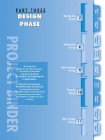
The Distribution of Income

I

n Part 5, we examine how a market economy distributes its income, using the price
mechanism, with the prices of the inputs to the production process determined by supply and demand; that is, we investigate what determines the share of total output that
goes to workers, to landowners, to investors, etc. We will see that the market assigns a
central role to the marginal productivity of each of these recipients—how much of a marginal contribution each makes to the economy’s total output.
In Chapter 19, we will study the payments made for the use of capital (interest), land
(rent), and the reward to entrepreneurs (profits). Because most people earn their incomes
primarily from wages and salaries, and because these payments constitute nearly threequarters of U.S. national income, our analysis of the payments to labor (wages) merits a
separate chapter (Chapter 20). In Chapter 21, we turn to some important problems in the
distribution of income—poverty, inequality, and discrimination.

C H A P T E R S
19 | Pricing the Factors
of Production

21 | Poverty, Inequality,

and Discrimination

20 | Labor and Entrepreneurship:
The Human Inputs

Copyright 2011 Cengage Learning, Inc. All Rights Reserved. May not be copied, scanned, or duplicated, in whole or in part.

Find more at www.downloadslide.com

Pricing the Factors of Production
Rent is that portion of the produce of the earth which is paid to the landlord
for use of the original and indestructible powers of the soil.
DAVI D RI CARD O ( 1772– 1823)

I

n Chapter 15, we noted that the market mechanism cannot be counted on to distribute income in accord with ethical notions of fairness, and we listed this as one of the
market’s shortcomings. But there is much more to say about how income is distributed
in a market economy.
The market mechanism distributes income through its payments to the factors of
production. Everyone owns some potentially usable factors of production—the inputs
used in the production process. Many of us have only our own labor; but some of us
also have funds that we can lend, land that we can rent, or natural resources that we
can sell at prices determined by supply and demand. The distribution of income in a
market economy is determined by the prices of the factors of production and by the
amounts that are employed. For example, if wages are low and unequal and unemployment is high, obviously many people will be poor.

Factors of production
are the broad categories—
land, labor, capital,
exhaustible natural
resources, and
entrepreneurship—into
which we classify the
economy’s different
productive inputs.

C O N T E N T S
PUZZLE: WHY DOES A HIGHER RETURN TO SAVINGS

REDUCE THE AMOUNTS SOME PEOPLE SAVE?

THE PRINCIPLE OF MARGINAL
PRODUCTIVITY
INPUTS AND THEIR DERIVED DEMAND
CURVES
INVESTMENT, CAPITAL, AND INTEREST
The Demand for Funds
The Downward-Sloping Demand Curve for Funds

PUZZLE RESOLVED: THE SUPPLY OF FUNDS
The Issue of Usury Laws: Are Interest Rates Too
High?

THE DETERMINATION OF RENT
Land Rents: Further Analysis
Generalization: Economic Rent Seeking
Rent as a Component of an Input’s Compensation
An Application of Rent Theory: Salaries of
Professional Athletes
Rent Controls: The Misplaced Analogy

PAYMENTS TO BUSINESS OWNERS:
ARE PROFITS TOO HIGH OR TOO LOW?
What Accounts for Profits?
Taxing Profits

CRITICISMS OF MARGINAL PRODUCTIVITY
THEORY
| APPENDIX | Discounting and Present Value

Copyright 2011 Cengage Learning, Inc. All Rights Reserved. May not be copied, scanned, or duplicated, in whole or in part.


Find more at www.downloadslide.com
398

Part 5

The Distribution of Income

PUZZLE:

Entrepreneurship is the
act of starting new firms,
introducing new products
and technological
innovations, and, in
general, taking the risks that
are necessary to seek out
business opportunities.

WHY DOES A HIGHER RETURN TO SAVINGS REDUCE
THE AMOUNTS SOME PEOPLE SAVE?

The rate of interest is the price one obtains by saving some money and lending it to others—for example, lending the money to a bank (by depositing the

money into a bank account) or lending the money to a corporation (by buying its bonds). We normally expect that a rise in the price of a loan (like the
price of anything else) will reduce the quantity demanded and increase the
quantity supplied. In fact, many people who save their money and lend it to others do
the opposite—they reduce the amount they lend when the rate of interest goes up. How
can that make sense?
The same puzzle affects other factors of production. For example, when wages, the
price of labor, rise, workers often decide to work less, perhaps taking longer vacations.
Why don’t they work more when pay is better? The explanation will be discussed later
in the chapter.
It is useful to group the factors of production into five broad categories: land, labor, capital, exhaustible natural resources, and a rather mysterious input called entrepreneurship.
In this chapter, we will look at two of them—the interest paid to capital and the rent of land.
But first, because there is a great deal of misperception about the distribution of income
among workers, suppliers of capital, and landlords, let’s see how much these three groups
actually earn. Of all the payments made to factors of production in the United States in
2006, interest payments accounted for about 4.5 percent; land rents were minuscule, making up only 0.7 percent; corporate profits accounted for 15 percent; and income of other
business proprietors made up 9.4 percent. In total, the payments to all the factors of production that we deal with in this chapter amounted to about 30 percent of national factor
income. Where did the rest of it go? The answer is that 70 percent of 2006 national factor
income consisted of employee compensation—that is, wages and salaries.1
There are many other serious misunderstandings about the nature of income distribution and about what government can do to influence it, and discussions of the subject are
often emotional. That’s because the distribution of income is the one area in economics in
which any one individual’s interests almost inevitably conflict with the interests of someone else. By definition, if I get a larger slice of the total income pie, then you end up with a
smaller slice. Still, as we will see in the next chapter, it is possible to get more for oneself
by increasing the size of the pie, and then everyone can benefit.

THE PRINCIPLE OF MARGINAL PRODUCTIVITY
The marginal physical
product (MPP) of an
input is the increase in
output that results from a
one-unit increase in the use

of the input, holding the
amounts of all other inputs
constant.
The marginal revenue
product (MRP) of an
input is the money value
of the additional sales that
a firm obtains by selling
the marginal physical
product of that input.

By now it should not surprise you that supply and demand determine the prices of inputs
as well as the prices of goods and services. The supply sides of the markets for the various
factors differ enormously, so we must discuss each factor market separately. We can use
one basic principle, the principle of marginal productivity, to explain how much of any input
a profit-maximizing firm will demand, given the price of that input. To review the principle, we must first recall two concepts from Chapter 7: marginal physical product (MPP)
and marginal revenue product (MRP).
Table 1 helps us review these two concepts in terms of Naomi’s Natural Farm, which has
to decide how much organic corn, priced at $10 per bag, to feed its chickens. The marginal

National Income and Product Accounts, U.S. Department of Commerce, Bureau of Economic Analysis, available at
. (Note: This calculation consists of the Bureau of Economic Analysis categories, Compensation of Employees, Proprietors’ Income with IVA and CCAdj., Rental Income of Persons with CCAdj., Corporate
Profits with IVA and CCAdj., and Net Interest and Miscellaneous Payments, all as a percentage of Net National
Factor Income.)
1

Copyright 2011 Cengage Learning, Inc. All Rights Reserved. May not be copied, scanned, or duplicated, in whole or in part.


Find more at www.downloadslide.com

Chapter 19

physical product (MPP) column tells us how many additional
pounds of chicken each additional bag of corn will yield. For
example, according to the table, the fourth bag increases output by 34 pounds. The marginal revenue product (MRP) column
tells us how many dollars this marginal physical product is
worth. In Table 1, we assume Naomi’s prized, natural chickens
sell at $0.75 per pound, so the MRP of the fourth bag of corn
is $0.75 per pound times 34 pounds, or $25.50 (last column of
the table).
The marginal productivity principle states that in competitive factor markets, the profit-maximizing firm will hire or
buy the quantity of any input at which the marginal revenue product equals the price of the input.

399

Pricing the Factors of Production

TABLE 1
Naomi’s Natural Farm Schedules for TPP, MPP, APP,
and MRP of Corn

(1)

(2)

(3)

Corn
Input
(Bags)

TPP:
Total
Physical
Product
(chicken, lbs)

MPP:
Marginal
Physical
Product
per Bag

0
1
2
3
4
5
6
7
8
9
10
11
12

0.0 lbs
14.0
36.0

66.0
100.0
130.0
156.0
175.0
184.0
185.4
180.0
165.0
144.0

14.0 lbs
22.0
30.0
34.0
30.0
26.0
19.0
9.0
1.4
25.4
215.0
221.0

The basic logic behind this principle is simple, as we saw
before. We know that the firm’s profit from acquiring an additional unit of an input is the input’s marginal revenue
product minus its marginal cost (which is the price of the additional unit of input). If the input’s marginal revenue product is greater than its price, it will pay the profit-seeking firm
to acquire more of that input because an additional unit of input brings the firm revenue that exceeds its cost. The firm
should purchase that input up to the amount at which diminishing returns reduce the MRP to the level of the input’s
price, so that further expansion yields zero further addition

to profit. By similar reasoning, if MRP is less than price, then the firm is using too much of
the input. We see in Table 1 that about seven bags is the optimal amount of corn for Naomi
to use each week, because an eighth bag brings in a marginal revenue product of only
$6.75, which is less than the $10 cost of buying the bag.
One corollary of the principle of marginal productivity is obvious: The quantity of any
input demanded depends on its price. The lower the price of corn, the more it pays the
farm to buy. In our example, it pays Naomi to use between seven and eight bags when the
price per bag is $10. But if corn were more expensive—say, $20 per bag—that high price
would exceed the value of the marginal product of either the sixth or seventh bag. It
would, therefore, pay the firm to stop at five bags of corn. Thus, marginal productivity
analysis shows that the quantity demanded of an input normally declines as the input price rises.
The “law” of demand applies to inputs just as it applies to consumer goods.

(4)
APP:
Average
Physical
Product
per Bag

(5)
MRP:
Marginal
Revenue
Product
per Bag

0.0 lbs
$10.50
14.0

16.50
18.0
22.50
22.0
25.50
25.0
22.50
26.0
19.50
26.0
14.25
25.0
6.75
23.0
1.05
20.6
24.05
18.0
211.25
15.0
215.75
12.0

INPUTS AND THEIR DERIVED DEMAND CURVES
We can, in fact, be much more specific about how much of each input a profit-maximizing
firm will demand. That’s because the marginal productivity principle tells us precisely
how to derive the demand curve for any input from its marginal revenue product (MRP)
curve.
Figure 1 graphs the MRP schedule from Table 1, showing the marginal revenue
product for corn (MRPc) rising and then declining as Naomi feeds more and more corn

to her chickens. In the figure, we focus on three possible prices for a bag of corn: $20,
$15, and $10. As we have just seen, the optimal purchase rule requires Naomi to keep
increasing her use of corn until her MRP begins to fall and eventually is reduced to the
price of corn. At a price of $20 per bag, we see that the quantity demanded is about
5.6 bags of corn per week (point A); at that point, MRP equals price. Similarly, if the
price of corn is $15 per bag, quantity demanded is about 6.8 bags per week (point B).
Finally, at a price of $10 per bag, the quantity demanded would be about 7.7 bags
per week (point C). Points A, B, and C are therefore three points on the demand
curve for corn. By repeating this exercise for any other price, we learn that because the

Copyright 2011 Cengage Learning, Inc. All Rights Reserved. May not be copied, scanned, or duplicated, in whole or in part.


Find more at www.downloadslide.com

MRP per Bag of Corn per Week

400

The Distribution of Income

Part 5

$26
24
22
20
18
16
14

12
10
8
6
4
2
0
–2
–4
–6
–8
–10
–12
–14
–16

profit-maximizing purchase of an input
occurs at the point where the MRP has fallen
down to the level of the input price,
A
D

The demand curve for any input is the
downward-sloping portion of its marginal
revenue product curve.2

B
C

0

1

2

3

4

5

6

7

8

Bags of Corn per Week

F I GURE 1
Marginal Revenue
Product Graph for
Naomi’s Natural Farm

MRP per Bag of Corn

The derived demand for
an input is the demand for
the input by producers as
determined by the demand

for the final product that the
input is used to produce.

$50
40
30
20
10
0

1

2

9

10

11

12

The demand for corn or labor (or for any
other input) is called a derived demand because it is derived from the underlying demand for the final product (poultry in this
case). For example, suppose that a surge in demand drives organic chicken prices to $1.50
per pound. Then, at each level of corn usage,
the marginal revenue product will be twice
as large as when poultry brought $0.75 per
pound. This effect appears in Figure 2 as an
upward shift of the (derived) demand curve

for corn, from D0D0 to D1D1, even though the
marginal physical product curves have not
changed. Thus, an outward shift in demand
for poultry leads to an outward shift in the demand for corn.3 We conclude that, in general:

An outward shift in the demand curve for any commodity causes an outward shift of
the derived demand curve for all factors utilized in the production of that commodity.

Similarly, an inward shift in the demand curve for a commodity leads to inward shifts in
the demand curves for factors used in producing that commodity.
This completes our discussion of the demand side of the analysis of input pricing.
The most noteworthy feature of the discussion is the fact that the same marginal productivity principle serves as the foundation for the
demand schedule for each and every type of input. In
particular, as we will see in Chapter 20, the marginal
productivity principle serves as the basis for the deD1
termination of the demand for labor—that crucial input whose financial reward plays so important a role
in an economy’s standard of living. On the demand
side, one analysis fits almost all.
D0
The supply side for each input, however, entails a
very different story. Here we must deal with each of
the main production factors individually. We must do
D0
D1
so because, as we will see, the supply relationships of
3
5
6
7
8

9 10
4
the different inputs vary considerably. We begin with
interest payments, or the return on capital. First, we
Bags of Corn per Week
must define a few key terms.

F I GURE 2
A Shift in the Demand
Curve for Corn

Why is the demand curve restricted to only the downward-sloping portion of the MRP curve? The logic of the
marginal productivity principle dictates this constraint. For example, if the price of corn were $15.00 per bag,
Figure 1 shows that MRP 5 P at two input quantities: (approximately) 1.75 bags (point D) and 6.8 bags (point B).
Point D cannot be the optimal stopping point, however, because the MRP of a second bag ($16.50) is greater than
the cost of the third bag ($15.00); that is, the firm makes more money by expanding its input use beyond 1.5 bags
per week. A similar profitable opportunity for expansion occurs anytime P 5 MRP and the MRP curve slopes
upward at the current price. This must be so, because then an increase in the quantity of input used by the firm
will raise MRP above the input’s price. It follows that a profit-maximizing firm will always demand an input
quantity that is in the range where MRP is diminishing.
3
To make Figure 2 easier to read, the (irrelevant) upward-sloping portion and the negative portion of each curve
have been omitted.
2

Copyright 2011 Cengage Learning, Inc. All Rights Reserved. May not be copied, scanned, or duplicated, in whole or in part.


Find more at www.downloadslide.com
Chapter 19

401

Pricing the Factors of Production

INVESTMENT, CAPITAL, AND INTEREST
Although people sometimes use the words investment and capital as if they were interchangeable, it is important to distinguish between them. Economists define capital as
the inventory (or stock) of plant, equipment, and other productive resources owned by a
business firm, an individual, or some other organization. Investment is the amount by
which capital grows. A warehouse owned by a firm is part of its capital. Expansion of the
warehouse by adding a new area to the building is an investment. So, when economists
use the word investment, they do not mean just the transfer of money. The higher the
level of investment, the faster the amount of capital that the investor possesses grows.
The relation between investment and capital is often explained by the analogy of filling
a bathtub: The accumulated water in the tub is analogous to the stock of capital, whereas
the flow of water from the faucet (which adds to the tub’s water) is like the flow of investment. Just as the faucet must be turned on for more water to accumulate, the capital
stock increases only when investment continues. If investment ceases, the capital stock
stops growing (but does not disappear). In other words, if investment is zero, the capital stock does not fall to zero but remains constant (just as when you turn off the faucet
the tub doesn’t suddenly empty, but rather the level of the water stays the same).
The process of building up capital by investing and then using this capital in production can be divided into five steps, listed below and summarized in Figure 3:

Investment is the flow
of resources into the
production of new capital.
It is the labor, steel, and
other inputs devoted to the
construction of factories,
warehouses, railroads, and
other pieces of capital
during some period of time.

SOURCE: © The New Yorker Collection 1995, Robert Mankoff from
cartoonbank.com. All Rights Reserved.

Step 1. The firm decides to enlarge its stock of
capital.
Step 2. The firm raises the funds to finance its
expansion, either by tapping outside sources
such as banks or by holding onto some of its
own earnings rather than paying them out to
company owners.
Step 3. The firm uses these funds to hire the
inputs needed to build factories, warehouses,
and the like. This step is the act of investment.
Step 4. After the investment is completed, the
firm ends up with a larger stock of capital.
Step 5. The firm uses the capital (along with
other inputs) either to expand production or
to reduce costs. At this point, the firm starts
earning returns on its investment.

Capital refers to an
inventory (stock) of plant,
equipment, and other
(generally durable)
productive resources held
by a business firm, an
individual, or some other
organization.

“I can’t sleep. I just got this incredible craving for capital.”

Notice that investors put money into the investment process—either their own or funds
borrowed from others. Then, through a series of steps, firms transform the funds into
physical inputs suitable for production use. If investors borrow the funds, they must

FIGU R E 3
The Investment Production Process

1
Decide to increase
the capital stock

2
Raise
funds

3
Investment flow:
Buy inputs, use
them to build up
capital stock

4
Added
capital
stock

Other
inputs

5

Production

Initial
capital
stock

Copyright 2011 Cengage Learning, Inc. All Rights Reserved. May not be copied, scanned, or duplicated, in whole or in part.


Find more at www.downloadslide.com
402

Part 5

The Distribution of Income

Interest is the payment
for the use of funds
employed in the production
of capital; it is measured
as the percent per year of
the value of the funds tied
up in the capital.

someday return those amounts to the lender with some payment for their use. This payment
is called interest, and it is calculated as an annual percentage of the amount borrowed. For
example, if an investor borrows $1,000 at an interest rate of 12 percent per year, the annual

interest payment is $120.

The Demand for Funds
The rate of interest is the price at which funds can be rented (borrowed). Just like other factor prices, interest rates are determined by supply and demand.
On the demand side of the market for loans are borrowers—people or institutions that,
for one reason or another, wish to spend more than they currently have. Individuals or
families borrow to buy homes or automobiles or other expensive products. Sometimes, as
we know, they borrow because they want to consume more than they can afford, which
can get them into financial trouble. But often, borrowing makes good sense as a way to
manage their finances when they experience a temporary drop in income. It also makes
sense to borrow money to buy an item such as a home that will be used for many years.
This long product life makes it appropriate for people to pay for the item as it is used,
rather than all at once when it is purchased.
Businesses use loans primarily to finance investment. To the business executive who
borrows funds to finance an investment and pays interest in return, the funds really represent an intermediate step toward the acquisition of the machines, buildings, inventories,
and other forms of physical capital that the firm will purchase. The marginal productivity
principle governs the quantity of funds demanded, just as it governs the quantity of corn
demanded for chicken feed. Specifically:
Firms will demand the quantity of borrowed funds that makes the marginal revenue
product of the investment financed by the funds just equal to the interest payment
charged for borrowing.

One noteworthy feature of capital distinguishes it from other inputs, such as corn.
When Naomi feeds corn to her chickens, the input is used once and then it is gone. But a
blast furnace, which is part of a steel company’s capital, normally lasts many years. The
furnace is a durable good; because it is durable, it contributes not only to today’s production but also to future production. This fact makes calculation of the marginal revenue
product more complex for a capital good than for other inputs.
To determine whether the MRP of a capital good is greater than the cost of financing it
(that is, to decide whether an investment is profitable), we need a way to compare money
values received at different times. For, other things being equal, a dollar to be received in

2011 is worth less than a dollar in 2010 because the recipient of the 2010 dollar has an additional year in which to use it to earn more money; for example, he can lend it out for an
additional year and earn the additional interest. To make such comparisons between
money obtained at different dates, economists and businesspeople use a calculation procedure called discounting. We will explain discounting in detail in the appendix to this
chapter, but it is not necessary to master this technique in an introductory course. There
are really only two important attributes of discounting to learn here:
• A sum of money received at a future date is worth less than the same sum of money

received today.
• This difference in values between money today and money in the future is greater

when the rate of interest is higher.

We can easily understand why this is so. To illustrate our first point, consider what you could
do with a dollar that you received today rather than a year from today. If the annual rate of
interest were 10 percent, you could lend it out (for example, by putting it in a savings
account) and receive $1.10 in a year’s time—your original $1.00 plus $0.10 interest. For this
reason, money received today is worth more than the same number of dollars received later.
Now for our second point. Suppose the annual rate of interest is 15 percent rather than
the 10 percent in the previous example. In this case, $1.00 invested today would grow to

Copyright 2011 Cengage Learning, Inc. All Rights Reserved. May not be copied, scanned, or duplicated, in whole or in part.


Find more at www.downloadslide.com
Chapter 19

403

Pricing the Factors of Production

$1.15 (rather than $1.10) in a year’s time, which means that $1.15 received a year from
today would be equivalent to $1.00 received today, and so, when the interest rate is 15 percent, $1.10 a year in the future must now be worth less than $1.00 today. In contrast, when
the interest rate is only 10 percent per year, $1.10 to be received a year from today is equivalent to $1 of today’s money, as we have seen. This illustrates the second of our two
points.
The rate of interest is a crucial determinant of the economy’s level of investment. It
strongly influences the amount of current consumption that consumers will choose to
forgo in order to use the resources to build machines and factories that can increase the
output of consumers’ goods in the future. The interest rate is crucial in determining the allocation of society’s resources between present and future—an issue that we discussed in
Chapter 15 (pages 318–319). Let us see, then, how the market sets interest rates.

The Downward-Sloping Demand Curve for Funds
A rise in the price of borrowed funds, like a rise in the price of any item, usually decreases
quantity demanded. But when the money is used for investment by the firm the situation
is a little more complicated than the relation between price and a consumers’ good. The
two attributes of discounting discussed above help to explain the special reasons why the
demand curve for funds has a negative slope.
Recall that the demand for borrowed funds, like the demand for all inputs, is a derived
demand, derived from the desire to invest in capital goods. But firms will receive part—
perhaps all—of a machine or factory’s marginal revenue product in the future. Hence,
the value of the MRP in terms of today’s money shrinks as the interest rate rises. Why? Because a given future return on investment in a machine or factory becomes worth less (it
must be discounted more) when the rate of interest rises, as our illustration of the second
point about discounting showed. As a consequence of this shrinkage, a machine that appears to be a good investment when the interest rate is 10 percent may look like a terrible
investment if interest rates rise to 15 percent; that is, the higher the interest rate, the fewer
machines a firm will demand. That is so because investing in the machines would use up
money that could earn more interest in a savings account. Thus, the demand curve for
machines and other forms of capital will have a negative slope—the higher the interest
rate, the smaller the quantity that firms will demand.
As the interest rate on borrowing rises, more and more investments that previously
looked profitable start to look unprofitable. The demand for borrowing for investment
purposes, therefore, is lower at higher rates of interest.

The higher the interest rate, the less people and firms will
want to borrow to finance their investments.

The Derived Demand
Curve for Loans

D
Rate of Interest in Percent per Year

Note that, although this analysis clearly applies to a firm’s
purchase of capital goods such as plant and equipment, it may
also apply to the company’s land and labor purchases. Firms
often finance both of these expenditures via borrowed funds,
and these inputs’ marginal revenue products may accrue only
months or even years after the inputs have been bought and
put to work. (For example, it may take quite some time before
newly acquired agricultural land will yield a marketable crop.)
Thus, just as in the case of capital investments, a rise in the interest rate will reduce the quantity demanded of investment
goods such as land and labor, just as it cuts the derived demand for investment in plant and equipment.
Figure 4 depicts a derived demand schedule for loans, with
the interest rate on the vertical axis as the loan’s cost to a borrower. Its negative slope illustrates the conclusion we have just
stated:

FI GURE 4

D

0
Dollars Demanded per Year

Copyright 2011 Cengage Learning, Inc. All Rights Reserved. May not be copied, scanned, or duplicated, in whole or in part.


Find more at www.downloadslide.com
404

Part 5

The Distribution of Income

PUZZLE RESOLVED:

F I GURE 5
Equilibrium in the
Market for Loans

Rate of Interest in Percent per Year

D

7.5%

A

5.5

S

0

THE SUPPLY OF FUNDS

Somewhat different relationships arise on the supply side of the market for
funds—where the suppliers or lenders are consumers, banks, and other business firms. Funds lent out are usually returned to the owner (with interest)
only over a period of time. Loans will look better to lenders when they bear
higher interest rates, so the supply schedule for loans rather naturally may
be expected to slope upward—at higher rates of interest, lenders supply
more funds. Such a supply schedule appears as the curve SS in Figure 5, where we
also reproduce the demand curve, DD, from Figure 4. Here, the free-market interest
rate is 7.5 percent.
However, not all supply curves for funds slope uphill to the right like curve SS.
As we stated in the puzzle at the beginning of the chapter, sometimes a rise in the
interest rate (the price of loans that is the financial reward for saving) will lead
people to save less, rather than more. An example will help to explain the reason for
this apparently curious behavior, which, as we will see, can sometimes be sensible
behavior. Say Jim is saving to buy a $10,000 used tractor in three years. If he lends
money out at interest in the interim, suppose Jim must save $3,100 per year to reach
his goal. If interest rates were higher, he could get away with saving less than
$3,100 per year and still reach his $10,000 goal because
every year, with the higher interest, he would get larger
interest payments on his savings. Thus, Jim’s saving
S
(and lending) may decline as a result of the rise in interest rate. This argument applies fully only to savers, like
Jim, with a fixed accumulation goal, but similar considE
erations affect the calculations of other savers. So when
the rate of interest rises, some people save more but
some save less.
B
Generally, we expect the quantity of loans supplied

to rise at least somewhat when the interest reward rises,
so the supply curve will have a positive slope, like SS in
Figure 5. However, for reasons similar to those indicated in Jim’s example, the increase in the economy’s
D
saving that results from a rise in the interest rate is usually quite small. That is why we have drawn the supply
curve to be so steep. The rise in the amount supplied by
some lenders is partially offset by a decline in the
amounts lent by savers with fixed goals (like Jim, who
is putting money away to buy a tractor, or Jasmine, who
Dollars Lent per Year
is saving for an expensive camera).
Having examined the relevant demand and supply curves, we are now in a position
to discuss the determination of the equilibrium rate of interest. This is summed up in
Figure 5, in which the equilibrium is, as always, at point E, where quantity supplied
equals quantity demanded. We conclude, again, that the equilibrium interest rate on loans
is 7.5 percent in the example in the graph.

The Issue of Usury Laws: Are Interest Rates Too High?
People have often been dissatisfied with the market mechanism’s determination of interest rates. Fears that interest rates, if left unregulated, would climb to exorbitant levels have
made usury laws (which place upper limits on money-lending rates) quite popular in
many times and places. Attempts to control interest payments date back to biblical days,
and in the Middle Ages the influence of the church even led to total prohibition of interest
payments in much of Europe. The same is true today in Moslem countries. In the United
Copyright 2011 Cengage Learning, Inc. All Rights Reserved. May not be copied, scanned, or duplicated, in whole or in part.


Find more at www.downloadslide.com
Chapter 19

405

Pricing the Factors of Production

States, the patchwork of state usury laws was mostly dismantled during the 1980s when
the banking industry was deregulated.
Unscrupulous lenders often manage to evade usury laws, charging interest rates even
higher than the free-market equilibrium rate. Even when usury laws are effective, they interfere with the operation of supply and demand and, as we will demonstrate, they may
harm economic efficiency.
Look at Figure 5 again but, this time, assume it depicts the supply of bank loans to consumers. Consider what happens if a usury law prohibits interest rates higher than 5.5 percent per year on consumer loans. At 5.5 percent, the quantity supplied (point A in Figure 5)
falls short of the quantity demanded (point B). This means that many applicants for consumer loans are being turned down even though banks consider them to be creditworthy.
Who gains and who loses from this usury law? The gainers are the lucky consumers
who get loans at 5.5 percent even though they would have been willing to pay 7.5 percent.
The losers are found on both the supply side and the demand side: the consumers who
would have been willing and able to get credit at 7.5 percent but who are turned down at
5.5 percent, and the banks that could have made profitable loans at rates of up to 7.5 percent if there were no interest-rate ceiling.
This analysis explains why usury laws can be politically popular. Few people sympathize with bank stockholders, and the consumers who get loans at lower rates are, naturally, pleased with the result of usury laws. Other consumers, who would like to borrow
at 5.5 percent but cannot because quantity supplied is less than quantity demanded, are
likely to blame the bank for refusing to lend, rather than blaming the government for outlawing mutually beneficial transactions.
Concern over high interest rates can be rational. It may, for example, be appropriate to
combat homelessness by making financing of housing cheaper for poor people. Of course,
it may be much more rational for the government to subsidize the interest on housing for
the poor rather than to declare high interest rates illegal, in effect pretending that those
costs can simply be legislated away, as a usury ceiling tries to do.4

THE DETERMINATION OF RENT

Annual Rent per Acre

The factor of production we will discuss next is land. Rent, the payment for the use of
land, is another price that, when left to the market, often seems to settle at politically unpopular levels. Rent controls are a frequent solution. We discussed the effects of rent

controls in Chapter 4 (pages 72–73), and we will say a bit
more about them later in this chapter. Our main focus
here is the determination of rents by free markets.
S
D
The market for land is characterized by a special feature
on the supply side. Land is a factor of production whose total quantity supplied is (roughly) unchanging and virtually
unchangeable: The same quantity is available at every possible price. Indeed, classical economists used this notion as
E
$2,000
the working definition of land, and the definition seems to
fit, at least approximately. Although people may drain
swamps, clear forests, fertilize fields, build skyscrapers, or
convert land from one use (a farm) to another (a housing
development), human effort cannot change the total supply
S
of land by very much.
1,000
What does this fact tell us about how the market determines land rents? Figure 6 helps to provide an answer.
Acres of Land
The vertical supply curve SS means that no matter what

D

FI GURE 6
The law also sometimes concerns itself with discrimination in lending against women or members of ethnic minority groups. Strong evidence suggests the existence of sex and race discrimination in lending. For example, as
late as the nineteenth century, married women were often denied loans without the explicit permission of their
husbands, even when the women had substantial independent incomes.
4

Determination of Land
Rent in Littleville

Copyright 2011 Cengage Learning, Inc. All Rights Reserved. May not be copied, scanned, or duplicated, in whole or in part.


Find more at www.downloadslide.com
406

The Distribution of Income

Part 5

D1

Annual Rent per Acre

D0

$2,500
2,000

F I GURE 7
A Shift in Demand
with a Vertical
Supply Curve

Economic rent is the
portion of the earnings of a
factor of production that

exceeds the minimum
amount necessary to induce
that factor to be supplied.

the level of rents, there are only 1,000 acres of land in a
small hamlet called Littleville. The demand curve, DD,
S
slopes downward and is a typical marginal revenue
product curve, predicated on the notion that the use of
land, like everything else, is subject to diminishing reA
turns. The free-market price is determined, as usual, by
the intersection of the supply and demand curves at
E
point E. In this example, each acre of land in Littleville
rents for $2,000 per year. The first interesting feature of
this diagram is that, because quantity supplied is rigidly
fixed at 1,000 acres whatever the price, the market level
D1
of rent is entirely determined by the market’s demand
D0
S
side. This leads to the second special feature: Any shift
1,000
in the demand curve that raises (or lowers) it by X dollars will raise (or lower) the equilibrium price of land by
Acres of Land
precisely the same amount—X dollars.
If, for example, a major university relocates to Littleville,
attracting more people who want to live there, the DD
curve will shift outward, as depicted in Figure 7. Equilibrium in the market will shift
from point E to point A. The same 1,000 acres of land will be available, but now each acre

will command a rent of $2,500 per acre. The landlords will collect more rent, even though
society gets no more of the input—land—from the landlords in return for its additional
payment.
The same process also works in reverse, however. If the university shuts its doors and
the demand for land declines as a result, the landlords will suffer even though they did
not contribute to the decline in the demand for land. (To see this, simply reverse the logic
of Figure 7. The demand curve begins at D1D1 and shifts to D0D0.)
This discussion shows the special feature of rent that leads economists to distinguish it
from payments to other factors of production. An economic rent is an “extra” payment
for a factor of production (such as land) that does not change the amount of the factor that
is supplied. Society is not compensated for a rise in its rent payments by any increase in
the quantity of land it obtains. Economic rent is thus the portion of the factor payment that
exceeds the minimum payment necessary to induce that factor to be supplied.
As late as the end of the nineteenth century, the idea of economic rent exerted a powerful influence far beyond technical economic writings. American journalist Henry George
was nearly elected mayor of New York in 1886, running on the platform that all government should be financed by a “single tax” levied on landlords, who, he said, are the only
ones who earn incomes without contributing to the productive process. George said that
landlords reap the fruits of economic growth without contributing to economic progress.
He based his logic on the notion that landowners do not increase the supply of their factor of production—the quantity of land—when rents increase.

Land Rents: Further Analysis
If all plots of land were identical, our previous discussion would be virtually all there is to
the theory of land rent. But plots of land do differ—in geographical location, topography,
nearness to marketplaces, soil quality, and so on. The early economists, notably David
Ricardo, took this disparity into account in their analysis of rent determination—a
remarkable nineteenth-century piece of economic logic still considered valid today.
The basic notion is that capital invested in any piece of land must yield the same rate of
return per dollar invested as capital invested in any other piece that is actually in use. Why?
If it were not so, capitalist renters would bid against one another for the more profitable
pieces of land. This competition would go on until the rents they would have to pay for
these parcels were driven up to a point that eliminated their advantages over other parcels.

Suppose that a farmer produces a crop on one piece of land for $160,000 per year in
labor, fertilizer, fuel, and other nonland costs, whereas a neighbor who is no more efficient

Copyright 2011 Cengage Learning, Inc. All Rights Reserved. May not be copied, scanned, or duplicated, in whole or in part.


Find more at www.downloadslide.com
Pricing the Factors of Production

407

produces the same crop for $120,000 on a second piece of land. The rent on the second
parcel must be exactly $40,000 per year higher than the rent on the first, because otherwise production on one plot would be cheaper than on the other. If, for example, the rent
difference were only $30,000 per year, it would be $10,000 cheaper to produce on the second plot of land. No one would want to rent the first plot and every grower would instead bid for the second plot. Rent on the first plot would be forced down by the lack of
customers, and rent on the second plot would be driven up by eager bidders. These pressures would come to an end only when the rent difference reached $40,000, so that both
plots became equally profitable.
At any given time, some low-quality pieces of land are so inferior that it does not pay
to use them at all—remote deserts are a prime example. Any land that is exactly on the
borderline between being used and not being used is called marginal land. By this definition, marginal land earns no rent because if its owner charged any for it, no one would
willingly pay to use it.
We combine these two observations—that the difference between the costs of producing on any two pieces of land must equal the difference between their rents and that zero
rent is charged on marginal land—to conclude that

Marginal land is land that
is just on the borderline of
being used—that is, any
land the use of which
would be unprofitable if the
farmer had to pay even a
penny of rent.

Chapter 19

Rent on any piece of land will equal the difference between the cost of producing the
output on that land and the cost of producing it on marginal land.

That is, competition for the superior plots of land will permit the landowners to charge
prices that capture the full advantages of their superior parcels.
This analysis helps us to understand more completely the effects of an outward shift in
the demand curve for land. Suppose population growth raises demand for land. Naturally, rents will rise. But we can be more specific than this statement. In response to an outward shift in the demand curve, two things will happen:
• It will now pay to employ some land whose use was formerly unprofitable. The land that
was previously on the zero-rent margin will no longer be on the borderline, and
some land that is so poor that it was formerly not even worth considering will
now just reach the borderline of profitability. The settling of the American West illustrates this process strikingly. Land that once could not be given away is often
now very valuable.
• People will begin to exploit already-used land more intensively. Farmers will use more
labor and fertilizer to squeeze larger amounts of crops out of their acreage, as has
happened in recent decades. Urban real estate that previously held two-story
houses will now be used for high-rise buildings.
These two events will increase rents in a predictable fashion. Because the land that is
considered marginal after the change must be inferior to the land that was considered marginal previously, rents must rise by the difference in yields between the old and new marginal lands. Table 2 illustrates this point. In the table, we deal with three pieces of land: A,
a very productive piece; B, a piece that was initially considered only marginal; and C, a
piece that is inferior to B but nevertheless becomes
marginal when the demand curve for land shifts
TABLE 2
upward and to the right.
Nonrent Costs and Rent on Three Pieces of Land
The crop costs $80,000 more when produced on B
Total
than on A, and $12,000 more when produced on C

Nonland Cost
Rent
Type
of
of
Producing
than on B. Suppose, initially, that demand for the crop
Land
a
Given
Crop
Before
After
is so low that Farmer Jones does not plant crops in
field C. Farmer Jones is on the fence about whether to
A. A tract that was better than $120,000 $80,000 $92,000
plant crops in field B. Because field B is marginal, it is
marginal before and after
B. A tract that was marginal
200,000 0
12,000
just on the margin between being used and being left
before but is attractive now
idle—it will command no rent. We know that the rent
C. A tract that was previously
212,000 0
0
on field A will be equal to the $80,000 cost advantage
not worth using but is now
of A over B. Now suppose demand for the crop inmarginal

creases enough so that plot C becomes marginal land.

Copyright 2011 Cengage Learning, Inc. All Rights Reserved. May not be copied, scanned, or duplicated, in whole or in part.


Find more at www.downloadslide.com
408

Part 5

The Distribution of Income

Then field B commands a rent of $12,000, the cost advantage of B over C. Plot A’s rent
now must rise from $80,000 to $92,000, the size of its cost advantage over C, the newly marginal land.
In addition to the quality differences among pieces of land, a second influence pushes
land rents up: increased intensity of use of land that is already under cultivation. As farmers apply more fertilizer and labor to their land, the marginal productivity of the land increases, just as factory workers become more productive when more is invested in their
equipment. Once again, the landowner can capture this productivity increase in the form
of higher rents. (If you do not understand why, refer back to Figure 7 and recall that the
demand curves are marginal revenue product curves—that is, they indicate the amount
that capitalists are willing to pay landlords to use their land.) Thus, we can summarize the
theory of rent as follows:
As the use of land increases, landlords receive higher payments from two sources:
• Increased demand leads the community to employ land previously not good enough

to use; the advantage of previously used land over the new marginal land increases,
and rents go up correspondingly.
• Land is used more intensively; the marginal revenue product of land rises, thereby in-

creasing the ability of the producer who uses the land to pay rent.

Generalization: Economic Rent Seeking
Economists refer to the payments for land as “rents,” but land is not the only scarce input
with a fixed supply, at least in the short run. Toward the beginning of the twentieth century, some economists realized that the economic analysis of rent can be applied to inputs
other than land. As we will see, this extension yielded some noteworthy insights.
The concept of rent can be used to analyze such common phenomena as lobbying in the
U.S. Congress (attempts to influence the votes of members of Congress) by industrial
groups, lawsuits between rival firms, and battles over exclusive licenses (as for a television station). Such interfirm battles can waste very valuable economic resources—for

Supply and demand do not equalize prices for identical commodities offered by different sellers when the commodity, such as land,
cannot be transferred from one geographic market to another. In
2008, for example, retailers on the Avenue des Champs-Elysees in
Paris paid an average of $1,134 per square foot, per year. In comparison, shop space on Milan’s Via Montenapoleone cost $983 per
square foot each year, and retail real estate on New Bond Street in
London cost $810 per square foot per year. A fifteen-block stretch
of 5th Avenue, between Central Park and 42nd Street in New York
City, ranked as the most expensive retail real estate in the world, at
$1,850 per square foot in 2008.

SOURCE: Matt Woolsey, “World’s Most Valuable Addresses,” Forbes, December 22,
2008, />mw_1222realestate.html.

SOURCE: © Adina Tovy/Robert Harding/Jupiterimages

Land Prices Around the World

Copyright 2011 Cengage Learning, Inc. All Rights Reserved. May not be copied, scanned, or duplicated, in whole or in part.


Find more at www.downloadslide.com
Chapter 19

Pricing the Factors of Production

example, the time that executives, bureaucrats, judges, lawyers, and economists spend
preparing and battling court trials. Because this valuable time could have been used in
production, such activities entail large opportunity costs. Rent analysis offers insights into
the reasons for these battles and provides a way to assess what quantity of resources people waste as they seek economic rents for scarce resources.
How is economic rent—which is a payment to a factor of production above and beyond
the amount necessary to get the factor to make its contribution to production—relevant in
such cases? Gordon Tullock, an economist also trained in legal matters, first identified the
phenomenon of rent seeking as the search and battle for opportunities to charge or collect
those payments above and beyond the amount necessary to create the source of the income.
An obvious source of such rents is a monopoly license. For example, a license to operate the only television station in town will yield enormous advertising profits, far above
the amount needed for the station to operate. That’s why rent seekers swoop down when
such licenses become available. Similarly, the powerful lobby for U.S. sweetener producers, including corn and beet growers as well as cane sugar farmers, pressures Congress to
impede cane sugar imports, because free importation would cut prices (and rents) substantially. Such activities need not increase the quantities of product supplied, just as
higher rents do not increase the supply of land. That is why any resulting earnings are
called “rent” and why the effort to obtain such earnings that contribute nothing to output
is called “rent seeking.”
How much of society’s resources will be wasted in such a process? Rent-seeking theory
can give us some idea. Consider a race for a monopoly cable TV license that, once awarded,
will keep competing stations from operating. Nothing prevents anyone from entering the race
to grab the license. Anyone can hire the lobbyists and lawyers or offer the bribes needed in
the battle for such a lucrative license. Thus, although the cable business itself may not be
competitive, the process of fighting for the license can be very competitive.
Of course, we know from the analysis of long-run equilibrium under perfect competition (Chapter 10, pages 206–209) that in such markets, economic profits approximate
zero—in other words, revenues just cover costs. If owners expect a cable license to yield,
say, $900 million over its life in rent, then rent seekers (that is, the companies competing
to gain the license in the first place) are likely to waste something close to that amount as
they fight for the license.

Why? Suppose each of 10 bidders has an equal chance at winning the license. To each
bidder, that chance should be worth about $90 million—1 chance in 10 of getting $900 million. If the average bidder spends only $70 million on the battle, each firm will still value
the battle for the license at $90 million minus $70 million. This fact will tempt an eleventh
bidder to enter and raise the ante to, say, $80 million in lobbying fees, hoping to grab the
rent. This process of attraction of additional bidders stops only when all of the excess rent
available has been wasted on the rent-seeking process, so there is no further motivation
for still more people to bid.

Rent as a Component of an Input’s Compensation
We can use the concept of economic rent to divide the payment for any input into two
parts. The first part is simply the minimum payment needed to acquire the input—for
example, the cost of producing a ball bearing or the compensation people require in exchange for the unpleasantness, hard work, and loss of leisure involved in performing
labor. The owners of the input must be offered this first part of the factor payment if
they are to supply the input willingly. If workers do not receive at least this first part,
they will not supply their labor.
The second part of the payment is a bonus that does not go to every input, but only to
inputs of particularly high quality, like the payment to the owner of higher-quality land in
our earlier example. Payments to workers with exceptional natural skills are a good illustration of the generalized rent concept. Because these bonuses are like the extra payment
for a better piece of land, they are called economic rents. Indeed, like the rent of land, an increase in the amount of economic rent paid to an input may not increase the quantity of

Copyright 2011 Cengage Learning, Inc. All Rights Reserved. May not be copied, scanned, or duplicated, in whole or in part.

409


Find more at www.downloadslide.com
410

Part 5

The Distribution of Income

that input supplied. This second part of the payment—the economic rent—is pure gravy.
The skillful worker is happy to have it as an extra, but it is not a deciding consideration in
the choice of whether or not to work.

An Application of Rent Theory: Salaries of Professional Athletes
Professional athletes may seem to have little in common with plots of farmland. Yet to an
economist, the same analysis—the theory of economic rent—explains how the market arrives at the amounts paid to each of these “factors of production.” To understand why,
let’s look at a hypothetical basketball team, the Lost Lakers, and its seven-foot star center,
Dapper Dan. First, we must note that there is only one Dapper Dan. That is, he is a scarce
input whose supply is fixed just like the supply of land. Because he is in fixed supply, the
price of his services is determined in a way similar to that of land rents.
A moment’s thought shows how the general notion of economic rent applies both
to land and to Dapper Dan. The total quantity of land available for use is the same
whether rent is high, low, or zero; only limited payments to landlords are necessary to
induce them to supply land to the market. By definition, then, a considerable proportion of the payments to landholders for their land is economic rent—payments above
and beyond those necessary for landlords to provide land to the economy. Dapper
Dan is (almost) similar to land in this respect. His athletic talents are unique and cannot be reproduced. What determines the payment to such a factor? Because the quantity supplied of such a unique, nonreproducible factor is absolutely fixed (there’s only
one Dapper Dan), and therefore unresponsive to price, the analysis of rent that we
summarized in Figure 6 applies, and the position of the demand curve for Dapper
Dan’s services is determined by the superiority of his services over those of other
players.
Suppose the Lost Lakers team also includes a marginal player, Weary Willy, winner of
last year’s Least Valuable Player award. Willy earns the $50,000 per year necessary to obtain his services. Suppose also that if no other option were available, Dapper Dan would
be willing to play basketball for $50,000 per year, rather than working as a hamburger
flipper, the only other job for which he is qualified. But Dan knows he can do better than
that. He estimates, quite accurately, that his presence on the team brings in $10 million of
added revenue over and above what the team would obtain if Dan were replaced by
a player of Willy’s caliber. In that case, Dan and his agent ought to be able to obtain

$10 million more per year than is paid to Willy. As a result, Dan obtains a salary of
$10,050,000, of which $10 million is economic rent—exactly analogous to the previous
rent example involving different pieces of land of unequal quality. Note that the team
gets no more of Dapper Dan’s working time in return for the rent payment. (See “A-Rod:
Earning Lots of Economic Rent” on the facing page for a real-world example.)
Almost all inputs, including employees, earn some economic rent. What sorts of inputs
earn no rent? Only those inputs that can be provided by a number of suppliers at equal
and constant cost and with identical quality earn no rents. For instance, no ball-bearing
supplier will ever receive any rent on a ball bearing, at least in the long run, because any
desired number of them, of equal quality, can be produced by any of the competing suppliers at (roughly) constant costs and can contribute equal amounts to the profits of those
who use them. If one ball-bearing supplier tried to charge a price above their x-cent cost,
another manufacturer would undercut the first supplier and take its customers away.
Hence, the competitive price includes no economic rent.

Rent Controls: The Misplaced Analogy
Why is the analysis of economic rent important? Because only economic rent can be taxed
away without reducing the quantity of the input supplied. Here common English gets in
the way of sound reasoning. Many people feel, in effect, that the rent they pay to their landlord is economic rent. After all, their apartments will still be there if they pay $1,500 per
month, or $500, or $100. This view, although true in the short run, is quite shortsighted.

Copyright 2011 Cengage Learning, Inc. All Rights Reserved. May not be copied, scanned, or duplicated, in whole or in part.


Find more at www.downloadslide.com
Chapter 19

Pricing the Factors of Production

411

In case you think that our discussion of economic rent is mere academic theorizing, check out these numbers: In 2000, in a deal that
sent shock waves through the baseball establishment, shortstop
Alex Rodriguez signed a 10-year, $252-million contract with the
Texas Rangers. His salary of more than $25 million per year makes
him one of the highest-paid professional athletes in sports history.
It is safe to assume that most of his salary is economic rent—in
other words, he would still be willing to play baseball if no team
offered him much more than a far smaller amount.
Less than four years later, the Rangers, finding themselves unable to afford A-Rod’s huge salary, traded their superstar shortstop
to the New York Yankees—who can afford him. In fact, however,
the Rangers will still pay part of Rodriguez’s salary through the year
2010. But the saga continued: In October 2007, after the Yankees
failed to reach the playoffs, A-Rod opted out of his contract and
became a free agent. Six weeks later, he signed a new $275 million
10-year contract with the Yankees organization. That move paid
off for the Yankees—in 2009 they defeated the Philadelphia Phillies
to win the World Series.

Like the ball-bearing producer, the owner of a building cannot expect to earn economic
rent because too many other potential owners whose costs of construction are roughly the
same will also offer apartments if rents are high. If the market price temporarily included
some economic rent—that is, if price exceeded production costs plus the opportunity cost
of the required capital—other builders would start new construction that would drive the
price down. Far from being in perfectly inelastic (vertical) supply, like raw land, buildings
come rather close to being in perfectly elastic (horizontal) supply, like ball bearings. As we
have learned from the theory of rent, this means that builders and owners of buildings
cannot collect economic rent in the long run.
Because apartment owners collect very little economic rent, payments by tenants in a
free market must be just enough to keep those apartments on the market (the very definition of zero economic rent). If rent controls push these prices down, the apartments will
start disappearing from the market.5 Among other unfortunate results, we can therefore

expect rent controls to contribute to homelessness—though it is, of course, not the only influence behind this distressing phenomenon.

PAYMENTS TO BUSINESS OWNERS: ARE PROFITS TOO HIGH
OR TOO LOW?
We turn next to business profits, the discussion of which often seems to elicit more
passion than logic. With the exception of some economists, almost no one thinks that
profit rates are at the right level. Critics point accusingly to some giant corporations’
billion-dollar profits and argue that they are unconscionably high; they then call for
much stiffer taxes on profits. On the other hand, the Chambers of Commerce, National
Association of Manufacturers, and other business groups complain that regulations
None of this is meant to imply that temporary rent controls in certain locations cannot have desirable effects in
the short run. In the short run, the supply of apartments and houses really is fixed, and large shifts in demand
can hand windfall gains to landlords—gains that are true, if temporary, economic rents. Controls that eliminate
such windfalls should not cause serious problems. But knowing when the “short run” fades into the “long run”
can be tricky. “Temporary” rent control laws have a way of becoming rather permanent.

5

Copyright 2011 Cengage Learning, Inc. All Rights Reserved. May not be copied, scanned, or duplicated, in whole or in part.

SOURCE: © Jason Szenes/EPA/Landov

“A-Rod”: Earning Lots of Economic Rent


Find more at www.downloadslide.com
412

Part 5

The Distribution of Income

and “ruinous” competition keep profits too low, and they constantly petition Congress
for tax relief.
The public has many misconceptions about the nature of the U.S. economy, but probably none is farther from reality than popular perceptions of what American corporations earn in profits. Try the following experiment. Ask five of your friends who have
never had an economics course what fraction of the nation’s income they imagine is
pure profit to companies. Although the correct answer varies from year to year, business
profits in 2006 made up 12.4 percent of gross domestic product (GDP) (before taxes).6 A
comparable percentage of the prices you pay represents before-tax profit. Most people
think this figure is much, much higher (see “Public Opinion on Profits” on page 31 in
Chapter 2).
As you can see, economists are reluctant to brand factor prices as “too low” or “too
high” in some moral or ethical sense. Rather, they are likely to ask first: What is the market equilibrium price? Then they will ask whether there are any good reasons to interfere
with the market solution. This analysis, however, is not so easily applied to the case of
profits, because it is difficult to use supply-and-demand analysis when you do not know
which factor of production earns profit.
In both a bookkeeping sense and an economic sense, profits are the residual. They are
what remains from the selling price after all other factors have been paid.

But which production factor earns this reward? Which factor’s marginal productivity
constitutes the profit rate?

What Accounts for Profits?
Economic profit is the
total revenue of a firm
minus all of its costs,
including the interest
payments and opportunity
costs of the capital it
obtains from its investors.

Economic profit, as we learned in Chapter 10, is the amount a firm earns over and above
the payments for all inputs, including the interest payments for the capital it uses and the
opportunity cost of any capital provided by the owners of the firm. The payment that
firm owners receive to compensate them for the opportunity cost of their capital (and
that in common parlance is considered profit) is closely related to interest rates but is not
part of economic profit. In an imaginary (and dull) world in which everything was certain
and unchanging, capitalists who invested money in firms would simply earn the market
rate of interest on their funds. Profits beyond this level would be competed away. Payment for capital below this level could not persist, because capitalists would withdraw
their funds from firms and deposit them in banks. Capitalists in such a world would be
mere moneylenders.
But the real world is not at all like this. Some capitalists are much more than moneylenders, and the amounts they earn often exceed current interest rates by a huge margin. This substantial earning can be a rent, of the sort we have just been considering. But
now we are discussing other sources of profit, which are obtained in return for some
productive service by the recipient (see “Nimble Entrepreneurship: Snatching Victory
from the Jaws of Defeat” for an example). However, we can list three primary ways in
which profits above “normal” interest rate levels can be earned.

1. Monopoly Power If a firm can establish a monopoly with some or all of its products, even for a short while, it can use that monopoly power to earn monopoly profits. We
analyzed the nature of these monopoly earnings in Chapter 11.

2. Risk Bearing Firms often engage in financially risky activities, subjecting the capitalist investors in the firm (as well as its employees) to some financial peril. For example,
when a firm prospects for oil, it must drill exploratory wells hoping to find petroleum at

6
SOURCE: National Income and Product Accounts, U.S. Department of Commerce, Bureau of Economic Analysis,
available at .

Copyright 2011 Cengage Learning, Inc. All Rights Reserved. May not be copied, scanned, or duplicated, in whole or in part.

Find more at www.downloadslide.com
Chapter 19

413

Pricing the Factors of Production

“The path to entrepreneurial success is not always obvious. In fact, in
the case of Scale Computing of Indianapolis, failure was the springboard.
Jeff Ready, the chief executive of Scale Computing, and his business partners said they originally thought they would use the
artificial-intelligence technology they had developed at a previous
start-up company to recast stock prices and make a fortune as
hedge fund gurus.
But by the time they had built their ‘magic box,’ the economy
had turned grim and they were unable to raise the $100 million
they thought they needed. It was only after potential customers
rejected other software technology ideas that they realized their
device could be marketed as a more practical product: a data storage system. Two years later, the orders are pouring in.
Andrew Zacharakis, a professor of entrepreneurship at Babson
College outside Boston, said Scale Computing’s owners followed a
classic entrepreneurial path of shifting gears as necessary to seize
real, as opposed to perceived, opportunities.”

SOURCE: Image copyright Tatuasha, 2009. Used under license from
Shutterstock.com

Nimble Entrepreneurship: Snatching Victory from the Jaws of Defeat

SOURCE: Excerpted from Brent Bowers, “Finding the Path to Success by
Changing Directions,” The New York Times, September 9, 2009, accessed

online at .

the bottom. Of course, many such exploratory wells end up as dry holes, and the costs
then bring no return. Lucky investors, on the other hand, do find oil and are rewarded
handsomely—more than the competitive return on the firm’s capital. The extra income
pays the firm for bearing risk.
A few lucky individuals make out well in this process, but many suffer heavy losses.
How well can we expect risk takers to do, on the average? If 1 exploratory drilling out of
10 typically pays off, do we expect its return to be exactly 10 times as high as the interest
rate, so that the average firm will earn exactly the normal rate of interest? The answer is
that the payoff will be more than 10 times the interest rate if investors dislike gambling—
that is, if they prefer to avoid risk. Why? Because investors who are risk averse will not be
willing to put their money into a business that faces such long odds—10 to 1—unless the
market provides compensation for the financial peril.
In reality, nothing guarantees that things will always work out this way. Some people
love to gamble and tend to be overly optimistic. They may plunge into projects to a degree unjustified by the odds. Average payoffs to such gamblers in risky undertakings may
end up below the interest rate. The successful investor will still make a good profit, just
like the lucky winner in Las Vegas. The average participant, however, will have to pay for
the privilege of bearing risk.

3. Returns to Innovation The third major source of profits is perhaps the most important of all for social welfare. People who introduce new outputs or new production
methods or find new markets for the commodities that the firm sells are called innovative entrepreneurs. The first entrepreneur able to innovate and market a desirable new
product or employ a new cost-saving machine will garner a higher profit than what an
uninnovative (but otherwise similar) business manager would earn. Innovation differs
from invention. Whereas invention generates new ideas, innovation takes the next step
by putting the new idea into practical use. Businesspeople are rarely inventors, but they
are often innovators.
When an entrepreneur innovates, even if the new product or new process is not protected by patents, the entrepreneur will be one step ahead of competitors. If the market

Invention is the act of

generating an idea for a
new product or a new
method for making an old
product.
Innovation also includes
the next step, the act of
putting the new idea into
practical use.

Copyright 2011 Cengage Learning, Inc. All Rights Reserved. May not be copied, scanned, or duplicated, in whole or in part.


Find more at www.downloadslide.com
414

Part 5

The Distribution of Income

likes the innovation, the entrepreneur will be able to capture most of the sales, either by
offering customers a better product or by supplying the product more cheaply. In either
case, the entrepreneur will temporarily have some monopoly power as the competitors
weaken and will receive monopoly profit for the initiative.
And the benefit to the community can be substantial. Innovative entrepreneurs have
played a crucial role in recognizing promising inventions and ensuring that they are put
to productive use. They have contributed enormously to the rapid growth of per-capita
income and the flood of new products that have emerged in the past several centuries.
The crucial role of the entrepreneur will be discussed more fully in the following chapter,
which will complete the elements of the story of economic growth that was begun in
Chapter 16.

Taxing Profits
Thus, we can consider profits in excess of market interest rates to be the return on entrepreneurial talent. But this definition is not really very helpful, because no one can say
exactly what entrepreneurial talent is. Certainly we cannot measure it; nor can we teach
it in a college course, although business schools may try. We do not know whether the
observed profit rate provides more than the minimum reward necessary to attract entrepreneurial talent into the market. This relationship between observed profit rates and
minimum necessary rewards is crucial when we start to consider the policy ramifications of taxes on profits—a contentious issue, indeed.
Consider a profits tax levied on oil companies. If oil companies earn profits well
above the minimum required to attract entrepreneurial talent, those profits contain a
large element of economic rent. In that case, we could tax away these excess profits
(rents) without fear of reducing oil production. In contrast, if oil company profits do not
include economic rents, then a windfall profits tax can seriously curtail oil exploration
and, hence, production.
This example illustrates the general problem of deciding how heavily governments
should tax profits. Critics of big business who call for high, if not confiscatory, profits
taxes seem to believe that profits are mostly economic rent. If they are wrong—if, in fact,
most of the observed profits are necessary to attract people into entrepreneurial roles—
then a high profits tax can be dangerous. Such a tax would threaten the very lifeblood of
the capitalist system. Business lobbying groups claim, predictably enough, that current tax
policy creates precisely this threat. Unfortunately, neither group has offered much evidence
to support its conclusion.

CRITICISMS OF MARGINAL PRODUCTIVITY THEORY
The theory of factor pricing described in this chapter once again uses supply-demand
analysis. Factor pricing theory also relies heavily on the principle of marginal productivity to derive the shape and position of the demand curve for various inputs. Indeed, some
economists refer to the analysis (rather misleadingly) as the marginal productivity theory of
distribution, when it is, at best, only a theory of the demand side of the pertinent market.
Over the years, factor pricing analysis has been subject to attack on many grounds. One
frequent accusation, which is largely (but not entirely) groundless, is the assertion that
marginal productivity theory merely attempts to justify the income distribution that the

capitalist system yields—in other words, that it is a piece of pro-capitalist propaganda.
According to this argument, when marginal productivity theory claims that each factor is
paid exactly its marginal revenue product, it is only a sneaky way of saying that each factor is paid exactly what it deserves. These critics claim that the theory legitimizes the gross
inequities of the system—the poverty of many and the great wealth of a few.
This argument is straightforward but wrong. First, payments are made not to factors of
production, but rather to the people who happen to own them. If an acre of land earns

Copyright 2011 Cengage Learning, Inc. All Rights Reserved. May not be copied, scanned, or duplicated, in whole or in part.


Find more at www.downloadslide.com
Chapter 19

Pricing the Factors of Production

415

$2,000 because that is its marginal revenue product, it does not mean, nor is it meant to
imply, that the landlord deserves any particular payment, because he may even have acquired the land by fraud.
Second, an input’s MRP does not depend only on “how hard it works” but also on how
much of it happens to be employed—because, according to the “law” of diminishing returns, beyond some level of employment, the more of an input that is employed, the lower
its MRP. Thus, a factor’s MRP is not and cannot legitimately be interpreted as a measure
of the intensity of its “productive effort.” In any event, what an input “deserves,” in some
moral sense, may depend on more than what it does in the factory. For example, workers
who are sick or have many children may be considered more deserving, even if they are
no more productive than their healthy or childless counterparts.
On these and other grounds, no economist today claims that marginal productivity
analysis shows that distribution under capitalism is either just or unjust. It is simply
wrong to claim that marginal productivity theory is pro-capitalist propaganda. The marginal productivity principle is just as relevant to organizing production in a socialist society as it is in a capitalist one.
Other critics have attacked marginal productivity theory for using rather complicated

reasoning to tell us very little about the really urgent problems of income distribution. In
this view, it is all very well to say that everything depends on supply and demand and to
express this idea in terms of many complicated equations (many of which appear in more
advanced books and articles). But these equations do not tell us what to do about such serious distribution problems as malnutrition among the indigenous populations in Latin
America or poverty among minority groups in the United States.
Although it does exaggerate the situation somewhat, there is some truth to this criticism. We have seen in this chapter that the theory provides some insights into real policy
matters, though not as many as we would like. Later in the book, we will see that economists do have useful things to say about the problems of poverty and underdevelopment,
but very little of what we can say about these issues arises out of marginal productivity
analysis.
Perhaps, in the end, what should be said for marginal productivity theory is this: As
the best model we have at the moment, marginal productivity theory offers us some valuable insights into the way the economy works, and until we find a more powerful model,
we are better off using the tools that we do have.

| SUMMARY |
1. A profit-maximizing firm purchases the quantity of any
input at which the price of the input equals its marginal
revenue product (MRP). Consequently, the firm’s demand curve for an input is (the downward-sloping portion of) that input’s MRP curve.
2. Investment in a firm is the amount that is added to
the firm’s capital, which is its plant, equipment, inventory, and other productive inputs that tie up the company’s money.
3. Interest rates are determined by the supply of and demand for funds. The demand for funds is a derived
demand, because these funds are used to finance
business investment whose profitability depends on
the demand for the final products turned out with the
aid of such investment. In this way, the demand for
funds depends on the marginal revenue productivity
of capital.
4. A dollar obtainable sooner is worth more than a dollar
obtainable later because of the interest that can be
earned on that dollar in the interim.

5. Increased demand for a good that needs land to produce
it will drive up the price of land either because inferior
land will be brought into use or because land will be
used more intensively.
6. Rent controls do not significantly affect the supply of
land, but they do tend to reduce the supply of buildings.
7. Economic rent is any payment to the supplier of a factor
of production that is greater than the minimum amount
needed to induce the factor to be supplied.
8. Factors of production that are unique in quality and difficult or impossible to reproduce will tend to be paid relatively high economic rents because of their scarcity.
9. Factors of production that are easy to produce at a constant cost and that are provided by many suppliers will
earn little or no economic rent.
10. Economic profits over and above the cost of capital are
earned (a) by exercise of monopoly power, (b) as payments for bearing risk, and (c) as the earnings of successful innovation.

Copyright 2011 Cengage Learning, Inc. All Rights Reserved. May not be copied, scanned, or duplicated, in whole or in part.


Find more at www.downloadslide.com
416

Part 5

The Distribution of Income

11. The desirability of increased taxation of profits depends
on the taxes’ effects on the supply of managerial talent.
If most profits are economic rents, then higher profits
taxes will have few undesirable effects. If most profits

are necessary to attract good managers or entrepreneurs
into the market, then higher profits taxes can weaken the
capitalist economy.

| KEY TERMS |
capital

401

derived demand

factors of production
400

innovation

economic profit 412

interest

economic rent 406

invention

entrepreneurship

investment

398

397

413

marginal land

407

marginal physical
product (MPP) 398

402

marginal revenue
product (MRP) 398

413
401

| TEST YOURSELF |
1. Which of the following inputs do you think include relatively large economic rents in their earnings?
a. Nuts and bolts
b. Petroleum
c. A champion racehorse
Use supply-demand analysis to explain your answer.
2. Three machines are employed in an isolated area. They
each produce 2,000 units of output per month, the first
requiring $20,000 in raw materials, the second $25,000,
and the third $28,000. What would you expect to be the
monthly charge for the first and second machines if the

services of the third machine can be hired at a price of
$9,000 per month? Which parts of the charges for the
first two machines are economic rent?
3. Economists conclude that a tax on the revenues of firms
will be shifted in part to consumers of the products of
those firms in the form of higher prices. However, they

believe that a tax on the rent of land usually cannot be
shifted and must be paid entirely by the landlord. What
explains the difference? (Hint: draw the supply-demand
graphs.)
4. Many economists argue that a tax on apartment buildings is likely to reduce the supply of apartments, but that
a tax on all land, including the land on which apartment
buildings stand, will not reduce the supply of apartments. Can you explain the difference? How is this
answer related to the answer to Test Yourself Question 3?
5. Distinguish between investment and capital.
6. Explain the difference between an invention and an innovation. Give an example of each.
7. What is the difference between interest and profit? Who
earns interest, in return for what contribution to production? Who earns economic profit, in return for what
contribution to production?

| DISCUSSION QUESTIONS |
1. A profit-maximizing firm expands its purchase of any
input up to the point where diminishing returns have
reduced the marginal revenue product so that it equals
the input price. Why does it not pay the firm to “quit
while it is ahead,” buying so small a quantity of the input that the input’s MRP remains greater than its price?
2. If you have a contract under which you will be paid
$10,000 two years from now, why do you become richer
if the rate of interest falls?

3. Do you know any entrepreneurs? How do they earn a
living? How do they differ from managers?
4. “Marginal productivity does not determine how much a
worker will earn—it determines only how many workers will be hired at a given wage. Therefore, marginal
productivity analysis is a theory of demand for labor,
not a theory of distribution.” What, then, do you think

determines wages? Does marginal productivity affect
their level? If so, how?
5. (More difficult) American savings rates are among
the lowest of any industrial country. This has caused
concern about our ability to finance new plants and
equipment for U.S. industry. Some politicians and others have advocated lower taxes on saving as a remedy.
Do you expect such a program to be very effective?
Why?
6. If rent constitutes only 2 percent of the incomes of
Americans, why may the concept nevertheless be
significant?
7. Litigation in which one company sues another often involves costs for lawyers and other court costs literally
amounting to hundreds of millions of dollars per case.
What does rent have to do with the matter?

Copyright 2011 Cengage Learning, Inc. All Rights Reserved. May not be copied, scanned, or duplicated, in whole or in part.


Find more at www.downloadslide.com
Chapter 19

417

Pricing the Factors of Production

| APPENDIX | Discounting and Present Value
Frequently in business and economic problems it is
necessary to compare sums of money received (or
paid) at different dates. Consider, for example, the
purchase of a machine that costs $11,000 and will yield
a marginal revenue product of $14,520 two years from
today. If the machine can be financed by a two-year
loan bearing 10 percent interest, it will cost the firm
$1,100 in interest at the end of each year, plus $11,000
in repayment of the principal (the amount originally
borrowed) at the end of the second year. (See the table
that follows.) Is the machine a good investment?
Costs and Benefits of Investing in a Machine

End of
Year 1
Benefits
Marginal revenue product of
the machine
Costs
Interest
Repayment of principal on loan
Total Cost

End of
Year 2

$1.00

$1.00
5 82.64 cents
2 5
11 1 i2
1.21
A similar analysis applies to money received three
years from today, four years from today, and so on.

1,100
0
1,100

1,100
11,000
12,100

The general formula for the present value of $1.00 to
be received N years from today when the rate of interest is i is

To illustrate the concept of present value, let us ask
how much $1 received a year from today is worth in
terms of today’s money. If the rate of interest is 10 percent, the answer is about 91 cents. Why? Because if we
invest 91 cents today at 10 percent interest, it will
grow to 91 cents plus 9.1 cents in interest 5 100.1 cents
in a year. That is, at the end of a year a payment of
$100 will leave the recipient about as well off as he
would have been if he had instead received $91 now.
Similar considerations apply to any rate of interest. In
general:
If the rate of interest is i, the present value of $1 to be

received in a year is

$1.00
11 1 i2

What about money to be received two years from
today? Using the same reasoning, and supposing the
interest rate is 10 percent so that 11i 5 1.1, $1.00 invested today will grow to $1.00 times (1.1) 5 $1.10
after one year and will grow to $1.00 times (1.1) times
(1.1) 5 $1.00 times (1.1)2 5 $1.21 after two years. Consequently, the present value of $1.00 to be received
two years from today is

$14,520

The process that has been invented for making the magnitudes of payments at different dates comparable to
one another is called discounting, or computing the
present value.

This is so, because in a year

$1.00
$1.00
$1.00
1
3i5
3 1 1 1 i 2 5 $1
11 1 i2
11 1 i2
11 1 i2

$0

The total costs of owning the machine over the twoyear period ($1,100 1 $12,100 5 $13,200) are less than
the total benefits ($14,520). But this is clearly an invalid comparison, because the $14,520 in future benefits is not worth $14,520 in terms of today’s money.
Adding up dollars received (or paid) at different dates
is a bit like adding apples and oranges.

$1.00
11 1 i2

will grow to the original amount plus the interest payment; that is,

$1.00
11 1 i2 N

The present value formula is based on the two variables that determine the present value of any future
flow of money: the rate of interest (i) and the amount
of time you have to wait before you get it (N).
Let us now apply this analysis to our example.
The present value of the $14,520 revenue is easy to
calculate because it all comes two years from today.
Because the rate of interest is assumed to be 10 percent (i 5 0.1), we have:

$14,520
1 1.1 2 2
$14,520
5
1.21
5 $12,000

Present value of revenues 5

The present value of the costs is a bit trickier in this
example because costs occur at two different dates.
The present value of the first interest payment is

$1,100
$1,100
5
5 $1,000
11 1 i2
1.1
The present value of the final payment of interest
plus principal is

$12,100
$12,100
5 $10,000
2 5
11 1 i2
1 1.1 2 2

Copyright 2011 Cengage Learning, Inc. All Rights Reserved. May not be copied, scanned, or duplicated, in whole or in part.


Find more at www.downloadslide.com
418

Part 5

The Distribution of Income

Now that we have expressed each sum in terms of
its present value, it is permissible to add them up. So
the present value of all costs is

Present value of costs 5 $1,000 1 $10,000

Comparing this figure to the $12,000 present value
of the revenues clearly shows that the machine really
is a good investment. We can use the same calculation
procedure for all investment decisions.

5 $11,000

| SUMMARY |
1. To determine whether a loss or a gain will result from a
decision whose costs and returns will come at several
different periods of time, we must discount all the figures represented by these gains and losses to obtain
their present value.

3. We then combine the present values of all the returns
and all the costs. If the sum of the present values of the
returns is greater than the sum of the present values
of the costs, then the decision to invest will promise a
net gain.

2. For discounting purposes, we use the present value formula for X dollars receivable N years from now with an
interest rate i:

Present value 5

X
11 1 i2 N

| KEY TERM |
discounting, or computing the
present value 417

| TEST YOURSELF |
1. Compute the present value of $1,000 to be received in
three years if the rate of interest is 11 percent.
2. A government bond pays $100 in interest each year for
three years and also returns the principal of $1,000 in the

third year. How much is it worth in terms of today’s
money if the rate of interest is 8 percent? If the rate of interest is 12 percent?

Copyright 2011 Cengage Learning, Inc. All Rights Reserved. May not be copied, scanned, or duplicated, in whole or in part.


Find more at www.downloadslide.com

Labor and Entrepreneurship:
The Human Inputs
Octavius (a wealthy young Englishman): “I believe most intensely in the dignity of labor.”
The chauffeur: “That’s because you never done any.”
GEORGE BERNARD SHAW, MA N A ND SUPER MA N , ACT I I

“O for a muse of fire that would ascend/ The brightest heaven of invention”

WI L L I AM SHAKE SP EARE, HENRY V, ACT I , S CE N E I

T

wo human factors of production can be credited with major contributions to a
nation’s production and economic growth—the labor force and the entrepreneurs.
The former contribute the physical and mental effort required for production. The latter
organize the workers’ efforts and ensure that they are provided with the capital and the
raw materials their activities require. They also find new ways to carry out these
processes, invent new products, and find new markets in which to sell them. We begin
this chapter with a discussion of the economics of labor activity, and then we will turn
to the entrepreneurs.

C O N T E N T S
PART 1: THE MARKETS FOR LABOR
PUZZLE: ENTREPRENEURS EARN LESS THAN MOST
PEOPLE THINK—WHY SO LITTLE?

WAGE DETERMINATION IN COMPETITIVE
MARKETS
The Demand for Labor and the Determination
of Wages
Influences on MRPL: Shifts in the Demand for Labor
Technical Change, Productivity Growth, and the
Demand for Labor
The Service Economy and the Demand for Labor

THE SUPPLY OF LABOR
Rising Labor-Force Participation
An Important Labor Supply Conundrum

The Labor Supply Conundrum Resolved

WHY DO WAGES DIFFER?
Labor Demand in General
Labor Supply in General
Investment in Human Capital
Teenagers: a Disadvantaged Group
in the Labor Market

UNIONS AND COLLECTIVE BARGAINING
Unions as Labor Monopolies
Monopsony and Bilateral Monopoly
Collective Bargaining and Strikes

PART 2: THE ENTREPRENEUR: THE OTHER
HUMAN INPUT

Fixed Costs and Public Good Attributes in Invention
and Entrepreneurship
Discriminatory Pricing of an Innovative Product
over Its Life Cycle
Negative Financial Rewards for Entrepreneurial
Activity?

PUZZLE RESOLVED: WHY ARE

ENTREPRENEURIAL EARNINGS SURPRISINGLY
LOW?

INSTITUTIONS AND THE SUPPLY

OF INNOVATIVE ENTREPRENEURSHIP

ENTREPRENEURSHIP AND GROWTH
The Entrepreneur’s Prices and Profits

Copyright 2011 Cengage Learning, Inc. All Rights Reserved. May not be copied, scanned, or duplicated, in whole or in part.


Find more at www.downloadslide.com
420

Part 5

The Distribution of Income

PART 1: THE MARKETS FOR LABOR

160

Index 1959 = 100

140
120
100
80
60
40
20
0
1909 1919 1929

F I GURE 1
Index of Trends in
Wages, Compensation,
and Work Hours,
1909–2005 (in Real,
Inflation-Adjusted
Terms)

PUZZLE:

ENTREPRENEURS EARN LESS THAN MOST PEOPLE THINK—WHY SO LITTLE?

The most obvious incentive for innovative
entrepreneurs to devote the time, effort, and
investment to innovative activity is the great
wealth and enormous prestige that success
in their undertaking appears to promise, as
in the case of superstar inventors such as Eli
Whitney, James Watt, Elias Singer, Thomas Edison, the
Wright Brothers, etc. But a healthy dose of reality may
be in order. Thomas Astebro* reports on the basis of
a sample of 1,091 inventions that, “only between
7–9 percent reach the market. Of the 75 inventions that
did, six received returns above 1400 percent, 60 percent obtained negative returns and the median was
negative” (p. 226).

SOURCE: © Library of Congress - digital version copyright
Science Faction / Getty Images

180

SOURCES: Constructed by the authors from data in U.S. Census Bureau, Historical
Statistics of the United States, Colonial Times to 1970 (Washington, D.C.: U.S.
Government Printing Office; 1975); Economic Report of the President (Washington, D.C.:
U.S. Government Printing Office; various years); and U.S. Bureau of Labor Statistics,
.

200

Labor costs account for by far the largest share of gross domestic product (GDP). As noted
in Chapter 19, the earnings of labor amount to almost three-quarters of national income.
Wages also represent the primary source of personal income for the vast majority of Americans. For more than a century, wages were the centerpiece of the American dream. In almost
every decade, the purchasing power of a typical worker’s earnings grew substantially, and
the U.S. working class evolved into a comfortable middle class—the envy of the world and
an irresistible lure for millions of immigrants. Then, something changed fundamentally in
ways economists do not yet fully understand.
Figure 1 shows that average
real wages (wages adjusted for
changes in the purchasing power
of the dollar) stopped their upward march around 1973 and, by
Hourly compensation
(wages plus benefits)
some (disputed) calculations,
even declined. In contrast, hourly
Hourly
wages
compensation (wages plus fringe
benefits) did not fall. Fringe benefits include things like health
insurance, retirement payments,

and education subsidies that emHours worked
ployers provide to their employper week
ees. But compensation growth did
slow markedly.1 The graph also
shows that average hours worked
per week have declined by almost
35 percent since the early 1900s,
1939 1949 1959 1969 1979 1989
2005
even when wages and compensation were increasing. (The big
drop in hours worked during the 1930s was a consequence of the Great Depression, and the
sharp rise in hours worked during the 1940s was attributable to World War II.) During most
of the 1990s, average hours worked per week remained virtually constant, then, after 2000,
started to drop slowly once again.

The sharp increases in compensation over the years reflect, at least in part, the rising cost of services such as
health care, rather than an increase in the quantity and quality of benefits provided to workers. We explored the
reasons for the rising costs of services in Chapter 15.

1

Copyright 2011 Cengage Learning, Inc. All Rights Reserved. May not be copied, scanned, or duplicated, in whole or in part.