Lecture Fundamentals of control systems: Chapter 8 - TS. Huỳnh Thái Hoàng
Bạn đang xem bản rút gọn của tài liệu. Xem và tải ngay bản đầy đủ của tài liệu tại đây (329.41 KB, 60 trang )
Lecture Notes
Fundamentals of Control Systems
Instructor: Assoc. Prof. Dr. Huynh Thai Hoang
Department of Automatic Control
Faculty of Electrical & Electronics Engineering
Ho Chi Minh City University of Technology
Email:
Homepage: www4.hcmut.edu.vn/~hthoang/
www4 hcmut edu vn/ hthoang/
6 December 2013
© H. T. Hoang - www4.hcmut.edu.vn/~hthoang/
1
Chapter 8
ANALYSIS OF
DISCRETE CONTROL SYSTEMS
6 December 2013
© H. T. Hoàng - www4.hcmut.edu.vn/~hthoang/
2
Content
Stability conditions for discrete systems
Extension of Routh-Hurwitz criteria
Jury
J
criterion
it i
Root locus
Steady
St d state
t t error
Performance of discrete systems
6 December 2013
© H. T. Hoàng - www4.hcmut.edu.vn/~hthoang/
3
Stability conditions for discrete systems
6 December 2013
© H. T. Hoàng - www4.hcmut.edu.vn/~hthoang/
4
Stability conditions for discrete systems
A system is defined to be BIBO stable if every bounded
input to the system results in a bounded output.
I s
Im
Stable
Res 0
I z
Im
Re s
| z | 1
Re z
1
z eTs
The region of stability for a
contin o s system
continuous
s stem is the
left-half s-plane
6 December 2013
Stable
The region of stability for a
di
discrete
t system
t
iis th
the
interior of the unit circle
© H. T. Hoàng - www4.hcmut.edu.vn/~hthoang/
5
Characteristic equation of discrete systems
Discrete systems described by block diagram:
R(s)
+
GC(z)
ZOH
G(s)
T
Y(s)
H(s)
Characteristic equation: 1 GC ( z )GH ( z ) 0
Discrete systems described by the state equation
x( k 1) Ad x( k ) Bd r ( k )
y ( k ) Cd x( k )
Characteristic equation: det( zI Ad ) 0
6 December 2013
© H. T. Hoàng - www4.hcmut.edu.vn/~hthoang/
6
Methods for analysis the stability of discrete systems
Algebraic stability criteria
The extension of the Routh-Hurwitz criteria
Jury’s
J ’ stability
t bilit criterion
it i
The root locus method
6 December 2013
© H. T. Hoàng - www4.hcmut.edu.vn/~hthoang/
7
The extension of the RouthRouth-Hurwitz criteria
6 December 2013
© H. T. Hoàng - www4.hcmut.edu.vn/~hthoang/
8
The extension of the Routh
Routh--Hurwitz criteria
Characteristic
C
a acte st c equat
equation
o o
of d
discrete
sc ete syste
systems:
s
a0 z n a1 z n 1 an 0
Im z
Im w
Region
R
i
off
stability
Re z
1
Region of
stability
1 w
z
1 w
Re w
The extension of the Routh-Hurwitz criteria: transform
zw,, and then apply
pp y the Routh – Hurwitz criteria to the
characteristic equation of the variable w.
6 December 2013
© H. T. Hoàng - www4.hcmut.edu.vn/~hthoang/
9
The extension of the Routh
Routh--Hurwitz criteria – Example
Analyze the stability of the following system:
R(s)
+
T 0.5
ZOH
G(s)
Y(s)
H(s)
3e s
Gi
Given
that:
th
t G( s)
s3
1
H ( s)
s 1
Solution:
Sol
tion
The characteristic equation of the system:
1 GH ( z ) 0
6 December 2013
© H. T. Hoàng - www4.hcmut.edu.vn/~hthoang/
10
The extension of the RouthRouth-Hurwitz criteria – Example (cont’)
s
G
(
s
)
H
(
)
s
3
e
GH ( z ) (1 z 1 )Z
G ( s)
s
( s 3)
s
3e
3
e
1
1
(1 z )Z
H (s)
( s 1)
s ( s 3)( s 1)
z ( Az B)
1 2
3(1 z ) z
( z 1)( z e 30.5 )( z e 10.5 )
(1 e 30.5 ) 3(1 e 0.5 )
A
0.0673
1
z ( Az B)
3(1 3)
Z
s3(s0.5 a)( s b)
( z 1)( z e aT )( z e bT )
3e 30.5 (1 e 0.5 ) e 0.5 (1 e
) aT
B
b(1 e 0).0346
a(1 e bT )
A
3(1 3)
ab(b a)
0.202 z 0.104
aeaT (1 e bT ) be bT (1 e aT )
GH ( z ) 2
z ( z 0.223)( zB 0.607) ab(b a)
6 December 2013
© H. T. Hoàng - www4.hcmut.edu.vn/~hthoang/
11
The extension of the RouthRouth-Hurwitz criteria – Example (cont’)
The characteristic equation:
1 GH ( z ) 0
0.202 z 0.104
1 2
0
z ( z 0.223)( z 0.607)
z 0.83z 0.135z 0.202 z 0.104 0
4
3
2
1 w
Perform the transformation: z
1 w
1 w
1 w
1 w
1 w
0.83
0.135
0.202
0.104 0
1 w
1 w
1 w
1 z w
0.202
0.104
GH ( z ) 2
G
z ( z 0.223)( z 0.607)
4
3
2
4
3
2
1.867 w 5.648w 6.354 w 1.52 w 0.611 0
6 December 2013
© H. T. Hoàng - www4.hcmut.edu.vn/~hthoang/
12
The extension of the RouthRouth-Hurwitz criteria – Example (cont’)
The Routh table
Conclusion: The system is stable because all the
terms in the first column of the Routh table are
positive
positive.
4
3
2
1.867 w 5.648w 6.354 w 1.52 w 0.611 0
6 December 2013
© H. T. Hoàng - www4.hcmut.edu.vn/~hthoang/
13
Jury stability criterion
6 December 2013
© H. T. Hoàng - www4.hcmut.edu.vn/~hthoang/
14
Jury stability criterion
Analyze the stability of the discrete system which has
the characteristic equation:
a0 z n a1 z n 1 an 1 z an 0
Jury table: consist of (2n+1) rows.
The first row consists of the coefficients of the
characteristic polynomial in the increasing index order.
The even row (any) consists of the coefficients of the
previous row in the reverse order.
The odd row i = 2k+1 (k1) consists (nk+1) terms,
the term at the row i column j defined by:
1 ci 2,1 ci 2,n j k 3
cij
ci 2,1 ci 1,1 ci 1,n j k 3
6 December 2013
© H. T. Hoàng - www4.hcmut.edu.vn/~hthoang/
15
Jury stability criterion (cont’)
Jury criterion statement: The necessary and
sufficient condition for the discrete system to be
stable
t bl is
i that
th t allll the
th first
fi t tterms off th
the odd
dd rows off th
the
Jury table are positive.
6 December 2013
© H. T. Hoàng - www4.hcmut.edu.vn/~hthoang/
16
Jury stability criterion – Example
Analyze the stability of the system which has the characteristic
equation:
3
2
5 z 2 z 3z 1 0
Solution: Juryy table
Row 1
Row 2
R
Row
3
Row 4
Row 5
Row 6
Row 7
Since all the first terms of the odd rows are positive, the system is stable.
6 December 2013
© H. T. Hoàng - www4.hcmut.edu.vn/~hthoang/
17
The root locus of discrete systems
6 December 2013
© H. T. Hoàng - www4.hcmut.edu.vn/~hthoang/
18
The root locus (RL) method
RL is a set of all the roots of the characteristic equation of
a system when a real parameter changing from 0 +.
Consider a discrete system which has the characteristic
equation:
N ((zz )
1 K
0
D( z )
Denote: G0 ( z ) K
N ( z)
D( z )
Assume that G0(z) has n poles and m zeros.
The rules for construction of the RL of continuous system
y
can be applied to discrete systems, except for the step 8.
6 December 2013
© H. T. Hoàng - www4.hcmut.edu.vn/~hthoang/
19
Rules for construction of the RL of discrete systems
Rule 1: The number of branches of a RL = the order of the
characteristic equation = number of poles of G0(z) = n.
Rule 2:
For K = 0: the RL begin at the poles of G0(z).
As
A K goes to
t + : m branches
b
h off th
the RL end
d att m zeros
of G0(z), the nm remaining branches goes to
approaching the asymptote defined by the rule 5 and
rule 6.
Rule 3: The RL is symmetric with respect to the real axis.
Rule
4: A point on the real axis belongs to the RL if the
t t l number
total
b off poles
l and
d zeros off G0(z)
( ) to
t its
it right
i ht is
i odd.
dd
6 December 2013
© H. T. Hoàng - www4.hcmut.edu.vn/~hthoang/
20
Rules for construction of the RL of discrete system (cont’)
Rule 5: The angles between the asymptotes and the real
axis are given by:
( 2l 1)
nm
Rule 6: The intersection between the asymptotes and
the real axis is a point A defined by:
poles zeros
OA
nm
(l 0,1,2,)
n
m
i 1
i 1
(pi and zi are
p
z
i i
nm
poles
l and
d zeros
of G0(z) )
Rule 7: : Breakaway / break-in points (or
break points for short), if any, are located in
the real axis and are satisfied the equation:
6 December 2013
© H. T. Hoàng - www4.hcmut.edu.vn/~hthoang/
dK
0
d
dz
21
Rules for construction of the RL of discrete system (cont’)
Rule 8: The intersections of the RL with the unit circle can
be determined by using the extension of the Routh-Hurwitz
criteria or by substituting z=a+jb (a2+b2 =1) into the
characteristic equation.
9: The departure angle of the RL from a pole pj (of
multiplicity 1) is given by:
Rule
m
j 1800 arg(( p j zi )
i 1
n
arg(( p
i 1,i j
j
pi )
The geometric
Th
t i form
f
off the
th above
b
formula
f
l is
i
j = 1800 + (angle from zi (i=1..m) to pj )
(angle
(
l pi (i=1..m,
(i 1
i≠j) to
t pj )
6 December 2013
© H. T. Hoàng - www4.hcmut.edu.vn/~hthoang/
22
The root locus of discrete systems – Example
Consider a discrete system described by a block diagram:
R(s)
+
T 0.1
ZOH
G(s)
( )
Y(s)
5K
G( s)
s( s 5)
Sketch the RL of the system when K=0+. Determine
the critical gain Kcr
Solution:The characteristic equation of the system:
1 G( z) 0
6 December 2013
© H. T. Hoàng - www4.hcmut.edu.vn/~hthoang/
23
The root locus of discrete systems – Example (cont’)
G(s)
5K
5
K
G ( z ) (1 z )Z
G ( s)
s
s ( s 5)
5K
1
(1 z )Z 2
s ( s 5)
0 . 5
) z (1 e 0.5 0.5e 0.5 )]
1 z[(0.5 1 e
K (1 z )
0 .5
2
5( z 1) ( z e )
0.021z 0.018
G( z) K
( z 1)( z 0.607)
1
Th characteristic
The
h
t i ti equation
ti :
0.021z 0.018
1 K
0 (*)
( z 1)( z 0.607)
aT
aT
aT
a
z
(
aT
1
e
)
z
(
1
e
aTe
)
Poles: p1 1 p2 Z 0.607
2
2
aT
s
(
s
a
)
a
(
z
1
)
(
z
e
)
Zeros: z1 0.857
6 December 2013
© H. T. Hoàng - www4.hcmut.edu.vn/~hthoang/
24
The root locus of discrete systems – Example (cont’)
The asymptotes:
(2l 1) (2l 1)
2 1
nm
poles zeros [1 0.607] ( 0.857)
OA 2.464
OA
nm
2 1
The breakaway/break-in points:
((*))
Then
( z 1)( z 0.607)
z 2 1.607 z 0.607
K
0.021z 0.018
0.021z 0.018
dK
0.021z 2 0.036 z 0.042
dz
(0.021z 0.018) 2
dK
0
dz
6 December 2013
z1 2.506
z2 0.792
© H. T. Hoàng - www4.hcmut.edu.vn/~hthoang/
25