Advances in Flight Control Systems Part 8 pptx
Bạn đang xem bản rút gọn của tài liệu. Xem và tải ngay bản đầy đủ của tài liệu tại đây (1.14 MB, 20 trang )
Design of Intelligent Fault-Tolerant Flight Control System for Unmanned Aerial Vehicles
127
airframe size by multiplying the scale-dependent constant value. The actuator-fixed fault
such as Lock-in-place, Hard-over and Float was adopted as the actuator fault model. (Jovan
D. Boskobic et al, 2005)
As the mission trajectory, turning above devastated district in constant height to observe
was applied. It is shown in Fig. 12. In this mission, the UAV flaw at the height of 30m in the
velocity of 20m/s and the constant wind was from +x direction. The gusts of wind was
expressed by changing the scale-dependent constant value of constant wind in 3 seconds.
(Kohichiroh Yoshida et al, 1994) In addition, not only the learned fault, left elevon-1 fault,
but also non-learned fault, rudder fault, was considered. The conditions of fault and gust are
represented in Table 2.
In the simulation, the proposed intelligent fault-tolerant flight control system and the flight
control system designed by MDM/MDP method were compared.
Fig. 12. Mission trajectory
Condition Time Direction
Gust1 15s From y minus
Failure 30s
Gust2 90s From x plus
Table 2. Conditions of disturbance
5.2 Simulation results
In this section, the simulation results under the condition shown in section 5.1 are
represented.
First, Figs. 13 to 19 respectively show the results under the conditions where the left elevon-
1 was fixed at 9 degree for the flight trajectory, the time history of bank angle, sideslip angle,
and actuator steerage. In addition, Table 3 shows the effective area.
Second, the results for detection, identification, and accommodation are shown. The output
of the detector and the identifier are respectively shown in Figs. 20 and 21. Figure 22 shows
the relationship between the fixed angle of broken elevon and the y-direction target value
Advances in Flight Control Systems
128
generated by the flight path generator. Moreover, the coherence functions between the
observed value and the estimated value for velocity u and angular velocity q are compared
under the conditions of a fault and gust of wind in Figs. 23 and 24.
Finally, Figs. 25 and 26 show the results under the condition where the rudder was fixed at -
8 degree for the flight trajectory and the time history of actuator steerage.
5.3 Evaluation
From the results in Figs. 13 to 19, we confirmed how each method deals with the fault in
which the elevon is fixed at the angle.
The conventional system generates a bank angle command and achieves a turning flight by
using an elevon. On the other hand, the proposed flight control system stabilizes the
airframe by using redundant elevon in horizontal flight as soon as the fault happens. After
that, it generates a sideslip angle command and achieves a turning flight by using a rudder.
-1000
0
1000
2000
-1000
0
1000
2000
0
20
40
y [m]
x [m]
-z [m]
Proposed System
Normal System
Proposed System
Normal System
Fig. 13. Flight trajectory (left elevon-1 fault)
0 50 100 150 200 250 300 350
-10
0
10
20
time [s]
bank angle [deg]
obs
cmd
Gust
Failure
Gust
Turning
Straight
Straight
Fig. 14. Time history of bank angle (normal system)
Design of Intelligent Fault-Tolerant Flight Control System for Unmanned Aerial Vehicles
129
0 50 100 150 200 250 300 350
-10
0
10
20
time [s]
bank angle [deg]
obs
cmd
Gust
Failure
Gust
Turning
Straight
Straight
Straight
Turning
Fig. 15. Time history of bank angle (proposed system)
0 50 100 150 200 250 300 350
-10
-5
0
5
10
time [s]
sideslip angle [deg]
obs
cmd
Gust
Failure
Gust
Turning
Straight
Straight
Fig. 16. Time history of sideslip angle (normal system)
Gust
Failure
Gust
0 50 100 150 200 250 300 350
-10
-5
0
5
10
time [s]
sideslip angle [deg]
obs
cmd
Turning
Straight
Straight
Straight
Turning
Fig. 17. Time history of sideslip angle (proposed system)
Advances in Flight Control Systems
130
0 50 100 150 200 250 300 350
-10
0
10
0 50 100 150 200 250 300 350
-10
0
10
0 50 100 150 200 250 300 350
-10
0
10
0 50 100 150 200 250 300 350
-10
0
10
0 50 100 150 200 250 300 350
-10
0
10
0 50 100 150 200 250 300 350
0
5
10
15
time[s]
350
obs
cmd
Gust
Failure
Gust
Fig. 18. Time history of actuator steerage (normal system)
0 50 100 150 200 250 300 350
-10
0
10
0 50 100 150 200 250 300 350
-10
0
10
0 50 100 150 200 250 300 350
0
5
10
15
time[s]
0 50 100 150 200 250 300 350
-10
0
10
0 50 100 150 200 250 300 350
-10
0
10
0 50 100 150 200 250 300 350
-10
0
10
350
obs
cmd
Gust
Failure
Gust
Fig. 19. Time history of actuator steerage (proposed system)
Design of Intelligent Fault-Tolerant Flight Control System for Unmanned Aerial Vehicles
131
0 10 20 30 40 50 60
0
1
2
3
time[s]
Flight Condition
Gust
Failure
Fig. 20. Output of detector neural network
Gust
Failure
0 10 20 30 40 50 60
-2
2
time[s]
0 10 20 30
40
50 60
-2
2
time[s]
0 10 20 30
40
50 60
-2
2
time[s]
0 10 20 30
40
50 60
-2
2
time[s]
0 10 20 30 40 50 60
-2
2
time[s]
1el
δ
2el
δ
1er
δ
2er
δ
r
δ
0 10 20 30 40 50 60
-2
2
time[s]
0 10 20 30
40
50 60
-2
2
time[s]
0 10 20 30
40
50 60
-2
2
time[s]
0 10 20 30
40
50 60
-2
2
time[s]
0 10 20 30 40 50 60
-2
2
time[s]
1el
δ
2el
δ
1er
δ
2er
δ
r
δ
0 10 20 30 40 50 60
-2
2
time[s]
0 10 20 30
40
50 60
-2
2
time[s]
0 10 20 30
40
50 60
-2
2
time[s]
0 10 20 30
40
50 60
-2
2
time[s]
0 10 20 30 40 50 60
-2
2
time[s]
1el
δ
2el
δ
1er
δ
2er
δ
r
δ
0 10 20 30 40 50 60
-2
2
time[s]
0 10 20 30
40
50 60
-2
2
time[s]
0 10 20 30
40
50 60
-2
2
time[s]
0 10 20 30
40
50 60
-2
2
time[s]
0 10 20 30 40 50 60
-2
2
time[s]
1el
δ
2el
δ
1er
δ
2er
δ
r
δ
Fig. 21. Output of identifier neural network
-10 -5 0 5 10
800
1000
1200
1400
degree of the locked angle[deg]
Target Value of Y direction [m]
-10 -5 0 5 10
800
1000
1200
1400
degree of the locked angle[deg]
Target Value of Y direction [m]
Proposed System
Normal System
Proposed System
Normal System
Fig. 22. Target value generated by flight path generator
Advances in Flight Control Systems
132
0 10 20 30 40 50
0
0.5
1
Frequency [Hz]
Coherence Function
Fault
Gust
Fig. 23. Coherence function, u
0 10 20 30 40 50
0
0.5
1
Frequency [Hz]
Coherence Function
Fault
Gust
Fig. 24. Coherence function, q
-1000
0
1000
2000
-1000
0
1000
2000
0
20
40
y [m]
x [m]
-z [m]
Fig. 25. Flight trajectory (rudder fault)
Design of Intelligent Fault-Tolerant Flight Control System for Unmanned Aerial Vehicles
133
0 50 100 150 200 250 300 350
-10
0
10
0 50 100 150 200 250 300 350
-10
0
10
0 50 100 150 200 250 300 350
-10
0
10
0 50 100 150 200 250 300 350
-10
0
10
0 50 100 150 200 250 300 350
-10
0
10
0 50 100 150 200 250 300 350
0
5
10
15
time[s]
350
obs
cmd
Gust
Failure
Gust
Fig. 26. Time history of actuator steerage (rudder fault)
Fault position Elevon Rudder
Range of movement [deg]
-13~13 -8~8
Effective area[deg]
-13~9 -8~8
Table 3. Effective area of proposed system
Advances in Flight Control Systems
134
The results in Figs. 13, 15, 17, and 19, confirm that the vibration motion is generated in the
horizontal flight after turning flight by using the proposed method. This vibration frequency
is about 0.067 Hz. This is because the resonation with the vibration occurs at the
longitudinal short cycle mode and the lateral-directional dutchroll mode when the turning
flight is changed to the horizontal flight in order to deal with the fault. However, this
vibration fits into the stable area of both an attack angle and a sideslip angle that is
established when designed and shown in section 4.6 as the termination conditions.
Therefore, the vibration is considered to be an allowable range.
From the results in Figs. 25 and 26, we confirmed that the proposed flight control system
generates a bank angle command and achieves a turning flight by using an elevon when a
rudder fault happens.
These results confirm that the proposed system can detect, identify and accommodate both
learned and non-learned faults.
From the simulation results, we confirmed that the proposed flight control system can
stabilize the airframe in fault situations shown in Table 3.
Figure 20 shows the output of a detector which means the evaluation value of a flight
condition. We confirmed that the detector can distinguish the fault from the gust of wind.
The flight control system can distinguish between the fault and the gusts from various
directions because a number of directional gusts are considered in the learning of neural
network. Figures 23 and 24 show that the gust has a wider range of frequency where the
coherence function takes the value of approximately 1 than the fault. If the disturbance is
estimated, the motion of the system is the same as the model assumed when the control
system is designed. On the other hand, the motion of the system with the fault is different
from the assumed model. Therefore, the proposed model-based detector can accurately
detect faults.
Figure 21 shows the output of an identifier which means the evaluation value of the fault
position. It was confirmed that the proposed identifier can identify the fault position
because only the broken actuator indicates the abnormal value.
Figure 22 shows the performance of a flight path generator. The horizontal axis indicates a
fixed angle of a broken elevon and the vertical axis indicates a new target value of y
direction that is calculated by the flight path generator. The results confirm that the higher
the level of a fault, the gentler the turning based on a new target value generated by the
flight path generator. In this research, the actuator error between the stable and the broken
conditions means the fault level. Moreover, the error from a mission trajectory is considered
in the evaluation function. Therefore, the proposed flight control system can generate a
suitable target value of turning in accordance with the situation.
The proposed flight control system focuses on the change in dynamics caused by a fault. It is
designed by considering the elevon fault that enormously influences the airframe because
an elevon plays the roles of both an aileron and an elevator. The simulation results confirm
the proposed system can perform well in both learned and non-learned fault situations.
6. Conclusion
This research aimed at proposing an intelligent fault-tolerant flight control system for an
unmanned aerial vehicle (UAV). In particular, the flight control system was developed that
Design of Intelligent Fault-Tolerant Flight Control System for Unmanned Aerial Vehicles
135
has estimator, detector, identifier, distributor, and flight path generator. The proposed
system distinguishes a fault from a disturbance like a gust of wind and automatically
generates a new flight path suited to the fault level. To verify the effectiveness of the
proposed method, a six-degree-of-freedom nonlinear simulation was carried out. In the
simulation, we assumed that the fault in left elevon-1, which was learned in designing each
neural network, or the fault in the rudder, which was not learned, would be generated in a
horizontal flight. The simulation results confirm that the proposed flight control system can
detect, identify and accommodate the fault and keep a flight stable. Moreover, the proposed
system can distinguish a fault from a gust and keep a flight stable automatically. It is
expected that the proposed design method can be used in broader flight areas by expanding
the learning area.
7. References
Akihiko Shimura and Kazuo Yoshida, Non-Linear Neuro Control for Active Steering for
Various Road Condition, The Japan Society of Mechanical and Engineers, Vol. 67, No.
654(2001), pp. 407-413.
Brian L. Steavens and Frank L. Lewis, Aircraft Control and Simulation 2
nd
Edition, JOHN
WILEY & SONS, INC. (2003)
Guillaume Ducard and Hans P. Geering, Efficient Nonlinear Actuator Fault Detection and
Isolation System for Unmanned Aerial Vehicles, AIAA, Journal of Guidance, Control,
and Dynamics, Vol. 31, No.1 (2008), pp. 225-237.
Jovan D. Boskovic, Sarah E. Bergstrom ,and Raman K. Mehra, Robust Integrated
Flight Control Design Under Failures, Damage, and State-Depenndent
Disturbances, AIAA, Journal of Guidance, Control, and Dynamics, Vol. 28, No.5 (2005),
pp. 902-916.
Kanichiro Kato, Akio Oya, and Kenzi Karasawa, Introduction of Aircraft Dynamics,
University of Tokyo Press, (1982).
Kohichiroh Yoshida, kazumichi Mototsuna and Yasushi Kumakura, Elementary knowledge
of marine technology, Seizandou,(1994)
Masaki Takahashi, Teruma Narukawa and Kazuo Yoshida, Robustness and Fault-Tolerance
of Cubic Neural Network Intelligent Control Method : Comparison with Sliding
Mode Control, The Japan Society of Mechanical and Engineers, Vol. 69, No. 682(2003),
pp. 1579-1586.
Mohammad Azam, Krishana Pattipati, Jeffrey Allanach, Scott Poll, and Ann Patterson-Hine,
In-flight Fault Detection and Isolation in Aircraft Flight Control Systems, Aerospace
Conference, 2005 IEEE, (2005), pp. 3555- 3565.
NAL/NASDA ALFLEX Group, Flight simulation model for Automatic Landing Flight
Experiment (Part I : Free Flight and Ground Run Basic Model), Technical Report of
National Aerospace Laboratory, Vol. 1252 (1994).
Taro Tsukamoto, Masaaki Yanagihara, and Takanobu Suito, Feasibility Study of
Lateral/Directional Control of Winged Re-entry Vehicle with Split Elevons,
Technical Report of National Aerospace Laboratory, Vol. 1379 (1999).
Advances in Flight Control Systems
136
Toshinari Shiotsuka, Kazusige Ohta, Kazuo Yoshida and Akio Nagamatsu, Identification
and Control of Four-Wheel-Steering Car by Neural Network, The Japan Society of
Mechanical and Engineers, Vol. 59, No. 559(1993), pp. 708-713.
Tsuyoshi Hatake, Junichiro Kawaguchi, and Tatsushi Izumi, Control in Aerospace,
CORONA PUBLISHING CO., LTD. (1999).
François Bateman
1
, Hassan Noura
2
and Mustapha Ouladsine
3
1
French Air Force Academy, Salon de Provence
2
United Arab Emirates University, Al-Ain
3
Paul Cezanne University, Marseille
1,3
France
2
United Arab Emirates
1. Introduction
Interest in Unmanned Aerial Vehicles (UAVs) is growing worldwide. Nevertheless there are
numerous issues that must be overcome as a precondition to their routine and safe integration
in military and civilian airspaces. Chief among these are absence of certification standards and
regulations addressing UAV systems, poor reliability record of UAV systems and operations.
Standards and regulations for airworthiness certification and flight operations in the military
and civilian airspaces are being studied (Brigaud, 2006). In this respect, the USAR standard
suggests a mishap rate of one catastrophic mishap per one million hours (Brigaud, 2006). To
reach such performances, upcoming technologies have the promise of significantly improving
the reliability of UAVs.
In this connection, a detailed study (OSD, 2003) shows that most of the breakdowns are due
to system failures such as propulsion, data link and Flight Control Systems (FCS). These
latter include all systems contributing to the aircraft stability and control such as avionics,
air data system, servo-actuators, control surfaces/servos, on-board software, navigation, and
other related subsystems. As regards FCS, it is recommended in (OSD, 2003) to incorporate
emerging technologies such as Self-Repairing Flight Control Systems (SRFCS) which have the
capability to diagnose and to repair malfunctions.
In this respect, Fault-tolerant control (FTC) are control systems that have the ability to
accommodate failures automatically in order to maintain system stability and a sufficient
level of performance. FTC are classified into passive and active methods. The analytical
fault-tolerant control operation can be achieved passively by the use of a control law designed
to guarantee an acceptable degree of performance in fault-free case and to be insensitive to
some faults. However, the passive methods are unsuitable to deal with a significant number
of faults. In particular, for an aircraft, it may be tricky to design an aprioricontroller able
to accommodate the whole of the faults affecting the control surfaces. By contrast, an active
FTC consists of adjusting the controllers on-line according to the fault magnitude and type, in
order to maintain the closed-loop performance of the system. To do so, a fault detection and
isolation (FDI) module which provides information about the fault is required (Noura et al.,
2009). Active FTC mechanisms may be implemented either via pre-computed control laws or
via on-line automatic redesign.
Active Fault Diagnosis and Major Actuator
Failure Accommodation: Application to a UAV
7
In this respect, FDI and FTC applied to aeronautical systems have received considerable
attention in the literature. However, regarding the control surface failures, some problematics
tackled in this chapter are underlined:
• severe failures are considered and the control surfaces may abruptly lock in any position
in their deflection range,
• each control surface being driven indenpendently, an actuator failure produces
aerodynamical couplings between the longitudinal and the lateral axis,
• the UAV is equipped with an autopilot which masks the failure effects,
• the aircraft studied is a small UAV and the control surface positions are not measured,
which makes the fault detection difficult,
• the control surfaces have redundant effects, which complicates the fault isolation,
• the FTC must take into account the bounds existing on the control surface deflections and
the flight envelope.
In this chapter, a nonlinear UAV model which allows to simulate assymetrical control surface
failures is presented (Bateman et al., 2009). In fault-free mode, a nominal control law based
on an Eigenstructure Assignment (EA) strategy is designed. As the control surface positions
are not measured, a diagnosis system is performed with a bank of observers able to estimate
the unkown inputs. However, as the two ailerons offert redundant effects, isolating a fault on
these actuators requires an active diagnosis method (Bateman et al., 2008a). In the last part,
a precomputed FTC strategy dedicated to accommodate for a ruddervator failure is depicted
(Bateman et al., 2008b).
All the models can be simulated with MATLAB-SIMULINK. Files and tutorial can be
downloaded at />2. Aircraft model
The aircraft studied in this paper and shown in Fig.1 is an inverted V-tail UAV. It is assumed
that its controls are fully indenpendent: δ
x
is the throttle, δ
ar
, δ
al
, δ
fr
, δ
fl
, δ
er
, δ
el
control the
right and left ailerons, the right and left flaps, the right and left inverted V tail control surfaces
respectively. These latter controls are named ruddervators because they combine the tasks
of the elevators and rudder. In the fault-free mode, the ailerons and the ruddervators are
known as the primary control surfaces, they produce the roll, the pitch and the yaw. As far as
the flaps are concerned, in the fault-free mode, they are only used to produce a lift increment
during takeoff and a drag increment during landing. They are known as the secondary control
surfaces.
It is assumed that each one of the primary control surfaces may lock at any arbitrary position
on its deflection range. To compensate for the fault, the FTC exploits the redundancies
provided by the remaining control surfaces. In this pespective, the UAV model has to consider
the aerodynamic effects produced by each control surface.
The following dynamic model of the aircraft is presented in the case of a rigid-body aircraft,
the weight m is constant and the centre of gravity c.g.isfixedposition.LetR
E
=
(
O, x
E
, y
E
, z
E
)
be a right-hand inertial frame such that z
E
is the vertical direction downwards the earth, ξ =
(
x, y, z) denotes the position of c.g.inR
E
.LetR
b
=
(
c.g., x
b
, y
b
, z
b
)
be a right-hand body fixed
frame for the UAV, at t
= 0 R
E
and R
b
coincide. The linear velocities μ =(u, v, w) and the
angular velocities Ω
=(p, q, r) are expressed in the body frame R
b
where p, q, r are roll, pitch
and yaw respectively. The orientation of the rigid body in R
E
is located with the bank angle
138
Advances in Flight Control Systems
Fig. 1. The RQ7A Shadow 200 UAV
φ, the pitch angle θ and the heading angle ψ. The transformation from R
b
to R
E
is given by a
transformation matrix T
bE
:
T
bE
=
⎛
⎝
cos θ cos ψ sin φ sin θ cos ψ
−cos φ sin ψ cos φ sin θ cos ψ + sin φ sin ψ
cos θ sin ψ sin φ sin θ sin ψ
+ cos φ cos ψ cos φ sin θ sin ψ −sin φ cos ψ
−sin θ sin φ cos θ cos φ cos θ
⎞
⎠
(1)
Forces F
R
b
x
, F
R
b
y
, F
R
b
z
acting on the aircraft are expressed in R
b
, they originate in gravity F
grav
,
propulsion F
prop
, and aerodynamic effects F
aero
. According to Newton’s second law:
⎛
⎝
˙
u
˙
v
˙
w
⎞
⎠
=
1
m
⎛
⎜
⎝
F
R
b
x
F
R
b
y
F
R
b
z
⎞
⎟
⎠
−
⎛
⎝
p
q
r
⎞
⎠
∧
⎛
⎝
u
v
w
⎞
⎠
(2)
where
∧ denotes the cross product. Let R
w
=
(
c.g., x
w
, y
w
, z
w
)
be the wind reference frame
where x
w
is aligned with the true airspeed V. The orientation of the body reference frame
in the wind reference frame is located with the angle of attack α and the sideslip β.The
transformation from R
b
to R
w
is given by a transformation matrix T
bw
:
T
bw
=
⎛
⎝
cos α cos β sin β sin α cos β
−cos α sin β cos β −sin α sin β
−sin α 0cosα
⎞
⎠
(3)
Furthermore, the aerodynamic state variables (V, α, β) and their time derivatives can be
formulated using T
bw
from μ (Rauw, 1993).
V
=
u
2
+ v
2
+ w
2
α = arctan
w
u
(4)
β
= arctan
v
√
u
2
+ w
2
For the sake of clarity, the forces are written in the reference frame where their expressions are
the simplest. They are transformed into the desired frame by means of the matrices T
bE
and
139
Active Fault Diagnosis and Major Actuator Failure Accommodation: Application to a UAV
T
bw
or their inverse.
F
grav
R
E
=
00g
T
F
prop
R
b
=
kρ
(z)
V
δ
x
00
T
(5)
F
aero
R
w
=
¯
qS
−C
D
C
y
−C
L
T
The model of the engine propeller is given in (Boiffier, 1998), ρ is the air density, k is a constant
characteristic of the propeller engine,
¯
q
=
1
2
ρV
2
and S denote the aerodynamic pressure and
a reference surface. The aerodynamic force coefficients are expressed as linear combination
of the state elements and control inputs. The values of these aerodynamic coefficients can be
found in the attached MATLAB files.
C
D
= C
D0
+
S
πb
2
C
2
L
+ C
Dδ
ar
|δ
ar
|+ C
Dδ
al
|δ
al
|+ C
Dδ
fr
|δ
fr
|+ C
Dδ
fl
|δ
fl
|+ C
Dδ
er
|δ
er
|+ C
Dδ
el
|δ
el
|
C
y
= C
yβ
β + C
yδ
ar
δ
ar
+ C
yδ
al
δ
al
+ C
yδ
fr
δ
fr
+ C
yδ
fl
δ
fl
+ C
yδ
er
δ
er
+ C
yδ
el
δ
el
(6)
C
L
= C
L0
+ C
Lα
α + C
Lδ
ar
δ
ar
+ C
Lδ
al
δ
al
+ C
Lδ
fr
δ
fr
+ C
Lδ
fl
δ
fl
+ C
Lδ
er
δ
er
+ C
Lδ
el
δ
el
The relationships between the angular velocities, their derivatives and the moments M
R
b
x
,
M
R
b
y
, M
R
b
z
applied to the aircraft originate from the general moment equation. J is the inertia
matrix.
⎛
⎝
˙
p
˙
q
˙
r
⎞
⎠
= J
−1
⎡
⎢
⎣
⎛
⎜
⎝
M
R
b
x
M
R
b
y
M
R
b
z
⎞
⎟
⎠
−
⎛
⎝
p
q
r
⎞
⎠
∧J
⎛
⎝
p
q
r
⎞
⎠
⎤
⎥
⎦
(7)
The moments are expressed in R
b
, they are due to aerodynamic effects and are modeled as
follows:
M
R
b
x
M
R
b
y
M
R
b
z
=
¯
qS
bC
l
¯
cC
m
bC
n
(8)
where
¯
c and b are the mean aerodynamic chord and the wing span. The aerodynamic moment
coefficients are expressed as a linear combination of state elements and control inputs as
C
l
= C
lβ
β + C
lp
bp
2V
+ C
lr
br
2V
+ C
lδ
ar
δ
ar
+ C
lδ
al
δ
al
+ C
lδ
er
δ
er
+ C
lδ
el
δ
el
+ C
lδ
fr
δ
fr
+ C
lδ
fl
δ
fl
(9)
C
m
= C
m0
+ C
mα
α + C
mq
¯
cq
2V
+ C
mδ
ar
δ
ar
+ C
mδ
al
δ
al
+ C
mδ
er
δ
er
+ C
mδ
el
δ
el
+ C
mδ
fr
δ
fr
+ C
mδ
fl
δ
fl
C
n
= C
nβ
β + C
np
bp
2V
+ C
nr
br
2V
+ C
nδ
ar
δ
ar
+ C
nδ
al
δ
al
+ C
nδ
er
δ
er
+ C
nδ
el
δ
el
+ C
nδ
fr
δ
fr
+ C
nδ
fl
δ
fl
Equations (6) and (9) make obvious the aerodynamic forces and moments produced by each
control surface. This is useful to model the fault effects and the redundancies provided by the
healthy control surfaces.
The FDI/FTC problem is first an attitude control problem, thus the heading angle ψ,thex and
y coordinates are not studied in the sequel.
With regard to the kinematic relations, the bank angle and the pitch angle time derivatives are
(Boiffier, 1998):
˙
φ
= p + q sin φ tan θ + r cos φ tan θ
˙
θ
= q cos φ − r sin φ
(10)
140
Advances in Flight Control Systems
The relationship between the time derivative of the position of the aircraft’s centre of gravity
ξ, the transformation matrix T
bE
and the linear velocities μ allows to write:
˙
z
= −u sin θ + v sin φ cos θ + w cos φ cos θ (11)
Let X
=(φθV αβpqrz)
T
the state vector and U =(δ
x
δ
ar
δ
al
δ
fr
δ
fl
δ
er
δ
el
)
T
the control vector. All the state vector is measured and Y is the measure vector.
From above, the model of the UAV can be written as a nonlinear model affine in the control
˙
X
= f (X)+g(X)U (12)
Y
= CX
Practically, the nonlinear aircraft model has been implemented with MATLAB in a sfunction.
In the fault-free mode, for a given operating point
{X
e0
, U
e0
},whereU
e0
denotes the trim
positions of the controls, the linearized model of the aircraft can be written as
˙x
= Ax + Bu (13)
y
= Cx (14)
2.1 Fault model
In the fault-free mode, the control surface deflections are constrained: asymmetrical aileron
deflections produce the roll control, pitch is achieved through deflecting both ruddervators
in the same direction and yaw is achieved through deflecting both ruddervators in opposite
direction. As for the flaps, their deflection is symmetrical.
The faults considered are stuck control surfaces. For t
≥ t
f
, the faulty control vector
U
f
(t)=U
f
,wheret
f
is the fault-time and U
f
are the stuck control surface positions. For
the simulations, a fault is modeled as a rate limiter response to a step. The slew rate is chosen
equal to the maximum speed of the actuators. Let U
h
be the remaining surfaces, then the state
equation (12) in faulty mode becomes:
˙
X
= f (X)+g
f
(X)U
f
+ g
h
(X)U
h
(15)
3. The nominal controller
A linear state feedback controller with reference tracking is designed. It is based on an
EA method which allows to set the aircraft handling qualities (Magni et al., 1997). This
method allows to set the modes of the closed-loop (CL) aircraft with respect to the standards
(MIL-HDBK-1797, 1997) and to decouple some state and control variables from some modes.
The design is based on the fault-free linearized model (13) which modal analysis shows that
the spiral mode is open-loop (OL) unstable.
Let
˜
Y
=
φβVz
the tracked vector and
˜
Y
ref
the reference vector. The autopilot is depicted
in figure 2 and the nominal control law is:
u
= Lζ + Kx (16)
where
˙
ζ
=
˜
Y
ref
−
˜
Y augments the state vector with the state variables which have to be tracked
to zero and
˙
ζ
=
ε
φ
ε
β
ε
V
ε
z
T
(17)
141
Active Fault Diagnosis and Major Actuator Failure Accommodation: Application to a UAV
✲ ✲ ✲ ✲
✻✻
✲
+
−
+
−
✛
K
L
♠
❄
✛
❄
+
−
X
e0
U
e0
X
UAV
✲
˜
C
˜
Y
re f
˜
Y
x
Fig. 2. The UAV control law
For a straight and level flight stage, Table 1 illustrates the EA strategy. A 0 means that the
mode and the state variable or the control are decoupled. On the contrary, an
× means that
they are coupled.
In the fault-free mode, the ruddervators produce the pitch and the yaw, thus the longitudinal
and the lateral axis are coupled. To take this into account, the autopilot is designed by
considering the complete linearized model of the aircraft (13). For example, a coupling has
been set between the spiral mode and the angle of attack which are a lateral mode and a
longitudinal state variable respectively. This is illustrated by the highlighted cells in Table 1.
This approach significantly differs from the classical method which consists in designing two
autopilots, one for the longitudinal axis, another one for the lateral axis. However, from the
FTC point of view, a control surface failure upsets the equilibrium of forces and moments
and produce significant couplings between longitudinal and lateral axis. Because of this, the
method adopted to design the nominal autopilot could be used to design the fault-tolerant
controllers. From (13), (16) and (17)
˙x
˙
ζ
=
A
+ BK BL
−
˜
C0
x
ζ
+
0
I
˜
Y
re f
(18)
with
˜
C
∈ R
4×9
and
˜
C(i, j)=1for{i, j} = {1, 1}, {2, 5}, {3, 3}, {4, 9} else
˜
C(i, j)=0.
Matrices K
∈ R
7×9
and L ∈ R
7×4
are computed in order to set the state space matrix’s
eigenvalues and eigenvectors in (18). These latter define the aircraft’s modes. The state space
matrix in (18) also writes:
A0
−
˜
C0
+
B
0
KL
= F + G
KL
(19)
Let λ
i
the i
th
eigenvalue (or closed-loop pole) corresponding to the eigenvector
−→
v
i
∈ R
13
,
next
F
+ G
KL
−→
v
i
= λ
i
−→
v
i
(20)
let
−→
w
i
=
KL
−→
v
i
∈ R
7
(21)
then
F
−λ
i
IG
−→
v
i
−→
w
i
=
−→
0 (22)
142
Advances in Flight Control Systems
mode short period phugoid throttle roll dutchroll spiral,ε
φ
ε
β
ε
V
,ε
z
OL poles −4.2 ± 9.6i −0.03 ±0.5i −0.0002 −21 −1.7 ±5.6i 0.073
CL poles −10 ±10i −2 ±2i −1 −100 −5 ±5i −1 ±.25i −1.5 −1 ±.5i
eigenvector
−→
v
1,2
−→
v
3,4
−→
v
5
−→
v
6
−→
v
7,8
−→
v
9,10
−→
v
11
−→
v
12,13
φ 0 0 0 × × × × ×
θ × × × 0 0 × 0 ×
V × × × 0 0 0 0 ×
α × × × 0 0 × 0 ×
β 0 0 0 × × × × ×
p 0 0 0 × × × × 0
q × × × 0 0 × 0 ×
r 0 0 0 × × × × 0
z × × × × × 0 × ×
ε
Φ
× × × × × × × ×
ε
β
× × × × × 0 × ×
ε
V
× × × × × × × ×
ε
z
× × × × × × × ×
δ
x
× × × × × × × ×
δ
ar
0 0 0 × × × × 0
δ
al
0 0 0 × × × × 0
δ
fr
0 0 0 0 0 0 0 0
δ
fl
0 0 0 0 0 0 0 0
δ
er
× × × × × 0 × ×
δ
el
× × × × × 0 × ×
Table 1. Eigenstructure assignment strategy, airspeed 25ms
−1
, height 200m
F
−λ
i
IG
is a 13 ×20 matrix and the size of its null space is equal to the number of control
inputs, here seven. In order to set the eigenvector structure (Table 1) while reducing the
solution space, some constraints are added. To hide the i
th
mode to the j
th
state variable
or control input, a mask is introduced such that
mask
i
=
1
0
···
0
j
1
0
···
20
0
(23)
In order to find a unique solution vector, for each eigenvalue λ
i
,sixmasksaredefinedandthe
system to solve writes
⎛
⎜
⎜
⎝
F
−λ
i
IG
mask
i1
mask
i6
⎞
⎟
⎟
⎠
−→
v
i
−→
w
i
=
−→
0 (24)
Let P
=
−→
v
1
−→
v
13
and Q
=
−→
w
1
−→
w
7
, then according to (21), matrices K and L write:
KL
= QP
−1
(25)
Fig. 4 shows the nominal autopilot functionning in the
[0s,16s] fault-free time interval.
4. Fault diagnosis
The class of faults addressed here are stuck control surfaces. However, the proposed diagnosis
system can also deal with actuator the loss of efficiency.
143
Active Fault Diagnosis and Major Actuator Failure Accommodation: Application to a UAV
To process for the faults, the diagnosis system could be realized by measuring the actuator
positions. This approach which requires potentiometers, wiring and acquisition board is
complex to implement and induces an increase of weight. Without these measurements, the
control inputs appear as unknown inputs which have to be estimated. This can be achieved
by the use of observers able to estimate the unknown inputs of a system.
In this connection, the problem of unknown, constant or slowy varying input estimation using
banks of Kalman filters is discussed in (Kobayashi & Simon, 2003), (Ducard & Geering, 2008).
The unknown inputs are declared as state variables, under the condition that the system is
observable, the problem consists in estimating an augmented state vector.
However, to catch for the actuator fault transients, the observer has to estimate time varying
inputs. Such an estimation is possible if these inputs are observable. The input observability
problem was addressed by Patton in (Hou & Patton, 1998) who gave some necessary and
sufficient conditions to prove input observability for linear time invariant systems with
unknown initial conditions.
As far as the observer is concerned, Xiong (Xiong & Saif, 2003) proposed an Unknown Input
Decoupled Functionnal Observer (UIDFO) which has no boundedness conditions as for time
varying inputs and does not require differentiation of the measured outputs.
The fact remains that control surfaces offer redundancies that make aileron failures not
isolable. In these conditions, an active diagnosis strategy has to be considered.
Input observability of the UAV is studied in subsection 4.1, the UIDFO is briefly described in
subsection 4.2 and a diagnosis system based on a bank of UIDFO is detailed in subsection 4.3.
The active diagnosis strategy is presented in subsection 4.4.
4.1 Input observability
Given, the linearized model (13).
Definition 1. The input u
(t) is said to be observable if y(t)=0 for t ≥ 0 implies u(t)=0 for t > 0
(Hou & Patton, 1998).
Let λ
∈ C , Σ
sys
and Σ
AC
refer to the system matrix and the observability pencil respectively,
they write:
Σ
sys
=
AB
CD
−λ
I0
00
and Σ
AC
=
A
C
−λ
I
0
(26)
Kroenecker’s theory of singular pencils shows that any pencil λM
−N with dimension m × n
can be brought into the canonical quasidiagonal form:
P(λM −N)Q =
⎛
⎜
⎜
⎝
λM
c
− N
c
×× ×
λI −N
f
××
λM
∞
−I ×
λM
r
− N
r
⎞
⎟
⎟
⎠
(27)
• P and Q are nonsingular constant matrices with dimensions m ×m and n × n.
• the finite eigenvalues are in the square and regular pencil λI
− J
f
and J
f
is in Jordan
canonical form. It is built with Jordan blocks J
f
i
with dimension i ×i.
• the infinite eigenvalues are in the square and regular pencil λJ
∞
− I and J
∞
is compound
with Jordan blocks J
∞
i
of size i ×i.
• λM
r
−N
r
is a singular pencil and has a block diagonal structure, each block takes the form
λM
r
i
− N
r
i
= λ
I
0
T
−
0
T
I
with dimension r
i+1
×r
i
. 0 stands for zero vector and 0
T
denotes its transpose. The r
i
are called Kroenecker’s row indices.
144
Advances in Flight Control Systems
• λM
c
−N
c
is a singular pencil and has a block diagonal structure, each block takes the form
: λM
c
j
−N
c
j
= λ
I0
−
0I
.Thec
j
×c
j+1
are called Kroenecker’s column indices.
This decomposition is applied to Σ
sys
and Σ
AC
. The following theorem contains a numerically
effective test for input observability:
Theorem 1. System (13) is input observable if and only if the block λM
c
sys
− N
c
sys
vanishes in
equation (27) and dim
(J
f
sys
)=dim( J
f
AC
) (Hou et Patton)(Hou & Patton, 1998).
Nevertheless, due to the numerical unreliability of the computation, this form is not suitable
and the staircase form, computed with the GUPTRI algorithm, is used to exhibit the
Kroenecker form (Demmel & Kågstrom, 1993).
All the state vector is measured and theorem 1 is applied to assess the ruddervator
observability. For this outpout vector, the matrix system and the observability pencil have
the following structures:
• Σ
AC
has no finite eigenvalue, nine singular pencils with Kronecker raw indice equal to
one,
• Σ
sys
has no finite eigenvalue, seven singular pencils with Kronecker raw indice equal to
one and two 2
×2 jordan blocks containing infinite eigenvalues.
According to theorem 1 the ruddervator positions are observable. With the same measured
outputs, theorem 1 is applied to assess the aileron observability. The matrix system and the
observability pencil have the following structure:
• Σ
AC
is unchanged
• Σ
sys
has no finite eigenvalue, one singular pencil with Kronecker column indice equal to
one, eight singular pencils with Kronecker raw indice equal to one and one 2
×2jordan
block containing infinite eigenvalues.
Due to the presence of the singular pencil with Kronecker column equal to one, the aileron
positions are not both observable. Thus, if one of the ailerons breaks down, the faulty control
is not isolable. This is depicted in Fig. 3 where a down lock position of the left aileron has the
same effects as a top lock position of the right aileron. In this case, an active diagnosis must
be used to discriminate the faulty control surface.
✲
❄
♠
−→
y
−→
z
✌
✌
p > 0p > 0
δ
er
δ
el
δ
ar
δ
al
δ
er
δ
el
δ
ar
δ
al
Fig. 3. Aerodynamic effects induced by right and left aileron failures
145
Active Fault Diagnosis and Major Actuator Failure Accommodation: Application to a UAV
4.2 The unknown input decoupled functional observer
In this part, results established in (Xiong & Saif, 2003) are recalled. The following dynamic
system driven by both known and unknown inputs is considered
˙x
= Ax + Bu + Gd (28)
y
= Cx
where x
∈ R
n
is the state vector, u ∈ R
m
is the known input vector, d ∈ R
is the unknown
input vector and y
∈ R
o
is the output vector. A, B, G and C are matrices with appropriate
dimensions, C and G are assumed to be full rank.
The UIDFO detailed in (Xiong & Saif, 2003) provides an estimation
ˆ
d of the unknown input
d and an estimation z of linear combination of state Tx. Theoretically, no boundedness
conditions are required for the unknown inputs and their derivatives.
˙z
= Fz + Hy + TBu + TG
ˆ
d (29)
ˆ
d
= γ(Wy −Ez) with γ ∈ R
∗+
Matrices F, H, T, W and E are all design parameters. in order to satisfy the following
conditions
⎧
⎪
⎪
⎪
⎪
⎨
⎪
⎪
⎪
⎪
⎩
FT
−TA + HC = 0 F is stable,
E
=(TG)
T
P with P solution of: PF + F
T
P = −Q
and Q, a semi-positive definite matrix,
ET
= G
T
T
T
PT = WC
rank
(TG)=rank(G)=
(30)
These matrices exist if and only if
(i) rank
(CG)=rank(G),
(ii) all unstable transmission zeros of system
(A, G, C) are unobservable modes of (A, C) .
To prove their existence and to calculate them, system (28) is transformed into "Special
Coordinate Basis" (SCB) (X.Liu et al., 2005).
4.3 Diagnosis system performed with a bank of UIDFO
The right aileron, the left aileron, the right ruddervator and the left ruddervator positions
are unknown. In order to estimate each one of these unknown input positions, a bank of
four UIDFOs is implemented. However, it has been proven above that the ailerons are not
both input observable. It means that, if one of these two controls is faulty, one of the two
estimations is wrong whereas the other is right, but in any case it is impossible to know which
one is which.
Let
ˆ
δ
ar
,
ˆ
δ
al
,
ˆ
δ
er
and
ˆ
δ
el
the positions estimated by each UIDFO, δ
ar
, δ
al
, δ
er
and δ
el
the known
control inputs computed by the nominal controller and
¯
δ
ar
,
¯
δ
al
,
¯
δ
er
and
¯
δ
el
the unknown
actual control surface positions. In the fault-free mode, the actual control surface positions are
equal to those computed by the controller and to their estimations. When an actuator breaks
down, the faulty actual control surface position is equal to its estimation but differs from that
computed by the controller. Residuals are obtained by processing the differences between the
positions computed by the controller with the estimated positions. The fault detection and
isolation process consists in monitoring residuals by comparing them with thresholds.
146
Advances in Flight Control Systems