Stable control of networked robot subject to communication delay, packet loss, and out-of-order delivery
Bạn đang xem bản rút gọn của tài liệu. Xem và tải ngay bản đầy đủ của tài liệu tại đây (1.29 MB, 21 trang )
Volume 36 Number 3
3
2014
Vietnam Journal of Mechanics, VAST, Vol. 36, No. 3 (2014), pp. 215 – 233
STABLE CONTROL OF NETWORKED ROBOT
SUBJECT TO COMMUNICATION DELAY, PACKET
LOSS, AND OUT-OF-ORDER DELIVERY
Manh Duong Phung∗ , Thuan Hoang Tran, Quang Vinh Tran
University of Engineering and Technology, VNU, Hanoi, Vietnam
∗
E-mail:
Received July 02, 2013
Abstract. Stabilization control of networked robot system faces uncertain factors caused
by the network. Our approach for this problem consists of two steps. First, the Lyapunov
stability theory is employed to derive control laws that stabilize the non-networked robot
system. Those control laws are then extended to the networked robot system by implementing a predictive filter between the sensor and controller. The filter compensates
influences of the network to acquire accurate estimate of the system state and consequently ensures the convergence of the control laws. The optimality of the filter in term
of minimizing the mean square error is theoretically proven. Many simulations and experiments have been conducted. The result confirmed the validity of the proposed approach.
Keywords: Networked robot, stabilization control, optimal filter.
1. INTRODUCTION
The stable movement from one point to another is essential for the efficient operation
of a control system and is basic for the development of real-world applications. In nonnetworked robot system, a number of researches have been introduced and the problem
of stabilization control has been solved in both theoretic and experimental aspects [1–3].
Networked robot systems (NRSs) however have differences. The occurrence of network
delay, packet loss and out-of-order delivery influences the accuracy of state estimation and
control so that directly applying previous control methods is no longer practical. Several
new approaches have been proposed.
Wargui et al. developed a stable controller for NRSs with nonholonomic constraints
[4]. Control laws that stabilize the system in delay-free scenario are first derived. They
are then extended to work with the time delay by adding a state estimator between the
system output and the controller. The estimator uses a multistep prediction mechanism
to predict the state that will be used for the controller. In [5], the maximum time delay
allowed at the control input without the loss of system stability is estimated. Based on
it, a single layered neural network is designed for the controller to control the robot with
unknown dynamics. In [6], Luck uses a time buffer which was longer than the worst delay
216
Manh Duong Phung, Thuan Hoang Tran, Quang Vinh Tran
to make the system to be time-invariant and then applied the classic control theory. In [7],
Xi and Tarn propose an event-based (non-time) control scheme to reduce the impact
of time delay on the system operation. This idea is expanded by Wang and Liu [8] in
which they introduced the telecommanding concept. In telecommanding, each command
is designed for an independent task and is defined with multiple events so that the robot
can deliberately respond to expected events while actively respond to unexpected events.
The main limitation of the proposed works is that they mainly focus on dealing with the
time delay, hardly address other issues such as the out-of-order delivery.
In this study, we address the problem of stabilization of NRS under the influence
of three inevitable network induced problems: the communication delay, packet loss, and
out-of-order delivery. The core of the scheme is the development of a new filter that is
able to predict the robot’s pose based on past observations so that control laws designed
for non-networked robot system can be used to stabilize the NRS. The filter is optimal
in sense that it minimizes the mean of the squared error. In addition, expansion of the
filter to nonlinear systems is also derived. The paper is organized as follows. Section 2
introduces the system model and formulates the control problem. Section 3 describes the
stabilization of non-networked robot system. The stabilization of NRS is introduced in
section 4. Section 5 presents the simulations, experiments, and discussions. Conclusions
are drawn in section 4.
2. SYSTEM MODEL AND PROBLEM FORMULATION
2.1. System Model
The robot considered in this study is the two-wheeled, differential-drive mobile robot
with non-slipping and pure rolling. The pose or state of the robot includes the position
of the wheel axis center (x, y) and the chassis orientation θ with respect to the x axis
(Fig. 1).
YG
XR
YR
R
k+n
ca
k u
Actuator
Process
k+n+1
Sensors
x
k+n+1 z
v(t)
Network
(Delay, Loss, Out of Order)
L
0
(t)
k+n+m+1
XG
Fig. 1. The robot’s pose and parameters
k
u
sc
k+n+1
z
Controller
Fig. 2. Model of a networked robot system
The kinematic models of the robot in continuous and discrete time domains in case
of no noise affected are given by
x˙ = v cos θ, y˙ = v sin θ, θ˙ = ω,
(1)
xk+1 = xk + Ts vk cos θk , yk+1 = yk + Ts vk sin θk , θk+1 = θk + Ts ωk ,
(2)
Stable control of networked robot subject to communication delay, packet loss, . . .
217
where Ts is the sampling period and v and ω are the tangent and angular velocities of the
robot, respectively. In practice, there always exist two kinds of noises in a robotic system
including the input and measurement noises. In this study, these noises are assumed to be
independent, zero-mean, and white-noise processes with normal probability distributions:
wk ∼ N(0, Qk ), vk ∼ N(0, Rk ), E(wi vjT ) = 0. This assumption is sufficient and widely
adopted due to the central limit theorem [9–12]. With the existence of noises, the robot
system can be described in state-space representation as follows.
Let x = [x y θ]T be the state vector. This state can be observed by a measurement
z. This measurement is described by a function h of the state vector and measurement
noise v. Denoting function (2) as f , with an input vector u = [v ω] and input disturbance
w, the representation of the robot in state space is given by
xk+1 = f (xk , uk , wk ),
zk = h(xk , vk ).
(3)
When distributing over communication networks, the robot becomes decentralized
and its functioning operation depends on a number of network parameters. The networks
are in general very complex and can greatly differ in their architecture and implementation
depending on the medium used, and on the applications they are meant to serve. In this
work, a network is modeled as a module between the process and controller which delivers
input signals and observation measurements with possible delay, loss, and out-of-order
(Fig. 2). The delay is assumed to be random but measurable at each sampling time. The
packet loss is modeled as a binary random variable λk defined as follows
λk =
1, if a packet arrives at time k
0, otherwise
(4)
The out-of-order packet with sequence number i arrived at time k(i < k) is modeled
as a delayed packet with the time delay
∆ti = ∆tk + (j − i)Ts ,
(5)
where ∆tk is the transfer time at time k and j is the sequence number of the last received
chronological packet.
Let n be the network delay (in number of sampling periods) between the controller
and the actuator, m be the network delay between the sensor and the controller, λca
k be the
binary random variable described the arrival of inputs from the controller to the actuator,
λsc
k be the binary random variable described the arrival of measurements from the sensor
to the controller. The system (3) becomes time-varying and can be rewritten as follows
xk = f (xk−1 , λca
k−n−1 uk−n−1 , wk−1 ),
sc
˜
zk = λsc
z
k−m k−m = λk−m h(xk−m , vk−m ).
(6)
2.2. Problem Formulation
Consider the control scenario shown in Fig. 3, with an arbitrary position and orientation of the robot and a predefined goal position and orientation. Let the difference
between the present pose (x, y, θ) and the final pose (x2 , y2 , θ2 ) given in the robot reference frame {XR , YR , θR } be the error vector, e = (x2 − x, y2 − y, θ2 − θ)T . The task of
218
Manh Duong Phung, Thuan Hoang Tran, Quang Vinh Tran
the controller layout is to find a control constraint, if it exists, of the tangent and angular
velocities such that the error e is driven toward zero: lim e(t) = 0.
t→∞
Y2
X2
O2
2
goal
Y
YR
(t)
YG
v(t)
XR
YG
X
O
start
0
OG
XG
Fig. 3. The goal of the controller
XG
Fig. 4. The robot poses and navigation variables
Our approach for this problem consists of two steps. First, control laws that stabilize
the non-networked robot system are derived. Then, a predictive filter is introduced to
extend those control laws to the NRS.
3. STABILIZATION OF NON-NETWORKED ROBOT SYSTEM
In (1), it can be seen that one degree of freedom of the system is constrained as
x˙ sin θ − y˙ cos θ = 0.
(7)
Thus, the system is nonholonomic. According to a work of Brockett [13], Cartesian
state-space representations of the robot cannot be asymptotically stabilized via smooth
and time invariant feedback laws. We therefore define a new coordinate system as shown
in Fig. 4.
The new coordinate system consists of three parameters (ρ, α, φ) called navigation
variables. Let OXY and O2 X2 Y2 be the local coordinate frames attached to the present
and final poses of the robot, respectively, ρ is then defined as the distance between O and
O2 , φ is the angular made by the vector connecting O and O2 and the vector connecting
O2 and x2 , and α is the angular made by the vector connecting O and O2 and the vector
connecting O and x
ρ = (x2 − x)2 + (y2 − y)2 ,
ϕ = a tan 2 (y2 − y, x2 − x) − θ2 ,
α = a tan 2 (y2 − y, y2 − x) − θ.
(8)
Without lost of generality, we assume that the goal desired pose of the robot is
(x2 , y2 , θ2 ) = (0, 0, 0) which can also be expressed by (ρ2 , α2 , ϕ2 ) = (0, 0, 0) (This can be
done by setting the origin of the global coordinate frame at the final position). Let wv and
wω be the input disturbances of the tangent and angular velocities, respectively. With the
existing of input disturbances, the kinematic model (1) is rewritten in navigation variable
Stable control of networked robot subject to communication delay, packet loss, . . .
219
domain (ρ, α, φ) as follows
ρ˙ = −(v + wv ) cos α,
α˙ = −(ω + wω ) + (v + wv ) sinρ α ,
ϕ˙ = (v + wω ) sinρ α .
(9)
The goal of the controller now is to establish smooth control laws that drive the
navigation variables (ρ, α, φ) toward zero.
By using Lyapunov theory, it is shown that (9) can be asymptotically stabilized
using the following control laws
v = (γ cos α)e,
ω = λα + γ cos ααsin α (α + hθ).
(10)
where γ, λ and h are the positive parameters [1, 14]. In discrete time domain, the control
laws are given by
vk = (γ cos αk )ek ,
(11)
ωk = λαk + γ cos ααk ksin αk (αk + hθk ).
Those control laws combined with a predictive filter are capable to stabilize the
NRS as presented in the next section.
4. STABILIZATION OF NETWORKED ROBOT SYSTEM
As shown in (6), the NRS is time-varying in which the control input at time k would
not reach the actuator until time k + n while the measurement at time k actually reflects
the system state at time k − m. Thus, in order to ensure the stabilization of control laws
(11) for NRS, the system state at time k + n need be estimated based on measurements
taken at time k − m, x
ˆ(k + n|k − m) (Fig. 5). This estimate will be used at the controller
to generate the control signal uk+n so that it will arrive to the actuator at time k + n
as expected. This approach is similar to [4] but we have developed a new state estimator
which is able to handle not only the network delay but also the packet loss and out-of-order
delivery. The filter called past observation-based predictive filter (PO-PF) is derived based
on the Kalman filter’s theory [9].
Actuator
k+n
uk+n
Process
k-m
x
Sensors
k-m
zk-m
k
zk-m
Network
State
Estimator
k
uk+n
^
Controller
xk+n
k
Fig. 5. NRS with the presence of a state estimator
220
Manh Duong Phung, Thuan Hoang Tran, Quang Vinh Tran
In this section, the standard Kalman filter is first briefly described. The derivation
of the PO-PF for linear systems is then introduced. Finally, the expansion of the PO-PF
for nonlinear systems is presented.
4.1. The standard Kalman filter
Consider the following discrete time linear stochastic system
xk = Ak−1 xk−1 + Bk−1 uk−1 + wk−1 ,
zk = Hk xk + vk ,
(12)
where k ∈ N, x and w ∈ Rn , z and v ∈ Rm , u ∈ Rl , A ∈ Rn × n , B ∈ Rn × l , H ∈ Rm × n ,
(x0 , w, v) are Gaussian, uncorrelated, white, with mean (¯
x, 0, 0) and covariance (P0 , Q, R)
respectively. The steps to calculate the Kalman filter can be summarized as follows [9]:
The time update equations (prediction phase)
x
ˆ−
ˆ+
k = Ak−1 x
k−1 + Bk−1 uk−1 ,
(13)
Pk−
(14)
=
+
Ak−1 Pk−1
ATk−1
+ Qk−1 ,
n
where x
ˆ−
k ∈ R is the priori state estimate at step k given knowledge of the process prior
to step k, and Pk− denotes the covariance matrix of the priori estimate error.
The data update equations (correction phase)
Kk = Pk− HkT [Hk Pk− HkT + Rk ]−1 ,
(15)
x
ˆ+
ˆ−
ˆ−
k =x
k + Kk [zk − Hk x
k ],
(16)
Pk+
= [I −
Kk Hk ]Pk− ,
(17)
n
where x
ˆ+
k ∈ R is the posteriori state estimate at step k given measurement zk , Kk is the
Kalman gain, and Pk+ is the covariance matrix of the posteriori estimate error.
4.2. The past observation-based predictive filter for linear NRSs
Consider the NRS described in (6). If functions f and h are linear, the system is
rewritten as
xk = Ak−1 xk−1 + λca
k−n−1 Bk−1 uk−n−1 + wk−1
(18)
= Ak−1 xk−1 + Bk−1 u
˜ k−n−1 + wk−1 ,
˜
zik = λsc
k−m zk−m
sc
= λsc
k−m Hk−m xk−m + λk−m vk−m
˜ i xi + v
=H
˜i ,
(19)
˜ k−m , v
where u
˜ k−n−1 , ˜
zik , H
˜k−m , and i are defined by the above equations. We can derive
the optimal filter to estimate the state of the stochastic linear system given in (18) and
(19) as follows.
Stable control of networked robot subject to communication delay, packet loss, . . .
221
Priori State Estimate at prediction phase
The priori estimate, x
ˆ−
k , is defined as the expectation of the state xk given all
measurements up to and including the last step k − 1. From (18), it is given by
x
ˆ−
uk−n−1 ) + E(wk−1 ).
k = E(xk ) = Ak−1 E(xk−1 ) + Bk−1 E(˜
(20)
As E(xk−1 ) is the posteriori state estimate at time k − 1, u
˜ k−n−1 is a known input,
and wk−1 is zero-mean, (20) becomes
x
ˆ−
ˆ+
˜ k−n−1 .
k = Ak−1 x
k−1 + Bk−1 u
(21)
At time k, the controller sends the input signal u
˜ k+n , (21) becomes
x
ˆ−
ˆ+
˜ k−1 .
k = Ak−1 x
k−1 + Bk−1 u
(22)
Priori Error Covariance
+
Let e−
k and ek be the priori and posteriori estimate errors, respectively
e−
ˆ−
k = xk − x
k,
(23)
e+
k
(24)
= xk −
x
ˆ+
k.
From (18) and (22), the covariance of the priori estimate error is given by
−T
Pk− = E(e−
k ek )
+T
T
T
= E(Ak−1 e+
k−1 ek−1 Ak−1 + wk−1 wk−1
(25)
+T
T
T
+ Ak−1 e+
k−1 wk−1 + wk−1 ek−1 Ak−1 )
+
= Ak−1 Pk−1
ATk−1 + Qk−1 .
Posteriori State Estimate at correction phase
From (19) the measurement ˜
zik received at time k would update the system state at a
previous time i rather than the present time k. Due to the network, this measurement could
not reach the estimator until time k. We therefore construct the data update equation of
the form
˜ ix
x
ˆ+
ˆ−
zik − H
ˆ−
(26)
i ),
k =x
k + Kk (˜
and recompute the Kalman gain and error covariance to ensure the optimality of the new
data update equation.
Kalman gain and Posteriori Error Covariance
Assume that the measurement is fused using (26) with an arbitrary gain Kk . The
covariance of the posteriori estimate error, Pk+ , is determined as
+T
Pk+ = E(e+
k ek )
−T
− −T
− T T
˜ i e− e−T
˜ T
= E[e−
˜ i Kk − Kk H
i k
k ek − ek ei (Kk Hi ) − ek v
− −T
− T T
T
˜
˜
˜
+ Kk Hi e e (Kk Hi ) + Kk Hi e v
˜ K − Kk v
˜i e−T
+
i i
−T
˜ i )T
Kk v
˜i ei (Kk H
+
i i
T T
Kk v
˜i v
˜i Kk ].
k
k
(27)
222
Manh Duong Phung, Thuan Hoang Tran, Quang Vinh Tran
Due to the independence between e− and v
˜, (27) can be simplified to
−T
− −T
− −T
˜ T
˜
Pk+ = E(e−
k ek ) − E(ek ei )(Kk Hi ) − Kk Hi E(ei ek )
˜ i E(e− e−T )(Kk H
˜ i )T + Kk E(˜
+ Kk H
vi v
˜iT )K T ]
=
Pk−
T
−L
i i
T T
˜
Hi Kk
˜ iL +
− Kk H
k
− ˜T T
˜
K k H i Pi H i K k +
(28)
˜iK T ,
Kk R
k
−T
where L = E(e−
i ek ).
As the matrix Kk is chosen to be the gain or blending factor that minimizes the
posteriori error covariance, this minimization is accomplished by taking the derivative of
the trace of the posteriori error covariance with respect to Kk , setting that result equal
to zero, and then solving for Kk . Applying this process to (28) obtains
∂tr(Pk+ )
˜ iT + Kk H
˜ i Pi H
˜ iT + Kk R
˜ i ) = 0,
= 2(−LT H
∂Kk
˜ iP −H
˜ iT + R
˜ i ]−1 .
˜ iT [H
⇔ Kk = LT H
i
(29)
(30)
Inserting (30) in (28) leads to a simpler form of Pk+
˜ i L.
Pk+ = Pk− − Kk H
(31)
In order to compute L, the priori state estimate at time k needs determining from
the estimate at time i. Through the time update (21) and the data update (26), e− becomes
e−
ˆ−
k = xk − x
k
= Ak−1 e+
k−1 − wk−1
˜ k−1 )e−
= Ak−1 [(I − Kk−1 H
k−1
(32)
+ Kk−1 v
˜k−1 ] − wk−1 .
After m updating steps, the estimation error becomes
−
e−
vi , . . . , v
˜k−1 ),
k = F ei + ξ1 (wi , . . . , wk−1 ) + ξ2 (˜
(33)
where
m
˜ k−j ),
Ak−j (I − Kk−j H
F =
(34)
j=1
˜. From (33) and the independence
and ξ1 and ξ2 are the functions of noise sequences w and v
−
between e and noise sequences, the covariance L becomes
−T
− T
L = E(e−
i e k ) = Pi F .
(35)
Substituting (35) in (31) and (30) yields
˜ iP −F T ,
Pk+ = Pk− − Kk H
i
(36)
˜ iT [H
˜ iP −H
˜ iT + R
˜ i ]−1 .
Kk = F Pi− H
i
(37)
and
Stable control of networked robot subject to communication delay, packet loss, . . .
223
Predictive state estimate at extrapolated phase
The extrapolated phase is added to predict the system state at time k + n from time
k. As there is no additional measurement, this phase is an open-loop propagation
x
ˆ−
ˆ+
˜ k+n−1 .
k+n = Ak+n−1 x
k+n−1 + Bk+n−1 u
(38)
• Remark 1: When the delay n and m is zero, F = I and the Kalman gain (37) reduces
to the standard form (15) and the error covariance (36) reduces to (17)
• Remark 2: Eq. (37) can be rewritten as
Kk = F Ki∗ ,
(39)
Ki∗
where
is the Kalman gain at time i of the standard Kalman filter (15). It turns out
˜ ˆ− ) in Eq. (26) can be normally updated to the posteriori
that the past residual (˜
z−
i
k Hi x
estimate at time k as at time i but the Kalman gain needs to be changed by the factor
F . This factor describes the relevant of the measurement updated at time i to the state
at time k.
• Remark 3: Eq. (26) can be rewritten as
i
x
ˆ+
ˆ−
ˆ−
(40)
i ).
k =x
k + λi Kk (zk − Hi x
It implies that if a measurement is not arrived (λi = 0), the estimator does not use
any information of the “dummy” observation to the estimate. It simply sets the posteriori
estimate to the value of the priori estimate.
4.3. The past observation-based predictive filter for nonlinear NRSs
Though the filter derived in previous section is capable for NRSs, the system has to
be linear. As practical robot systems are often nonlinear, further modification needs to be
accomplished. The main idea is the linearization of a nonlinear system around its previous
estimated states.
Performing a Taylor series expansion of the state equation around (ˆ
x+
˜ k−1 , 0)
k−1 , u
gives
∂f
∂f
(xk−1 − x
ˆ+
wk−1
k−1 ) + ∂w
∂x (ˆ
x+
(ˆ
x+
k−1 ,uk−1 ,0)
k−1 ,uk−1 ,0)
f (ˆ
x+
˜ k−1 , 0) + Ak−1 (xk−1 − x
ˆ+
k−1 , u
k−1 ) + Wk−1 wk−1
+
Ak−1 xk−1 + [f (ˆ
xk−1 , u
˜ k−1 , 0) − Ak−1 x
ˆ+
k−1 ] + Wk−1 wk−1
∗
∗
Ak−1 xk−1 + u
˜ k−1 + wk−1 ,
xk = f (ˆ
x+
˜ k−1 , 0) +
k−1 , u
=
=
=
(41)
∗
where Ak−1 , Wk−1 , u
˜ ∗k−1 , w
˜ k−1
are defined by the above equation. Similarly, the measurement equation is linearized around (ˆ
x−
i , 0) to obtain
∂h
x−
(xi − x
ˆ−
˜
zik = λi [h(ˆ
i , 0) + ∂x (ˆ
i )+
x−
i ,0)
−
−
˜
˜
˜
= h(ˆ
xi , 0) + Hi (xi − x
ˆi ) + Vi vi
˜ x− , 0) − H
˜ i xi + [h(ˆ
˜ ix
˜
=H
ˆ−
i
i ] + Vi vi
∗
∗
˜
= Hi xi + ε + v
˜ ,
i
i
∂h
vi ]
∂v (ˆ
x−
i ,0)
(42)
224
Manh Duong Phung, Thuan Hoang Tran, Quang Vinh Tran
∗
˜ i, H
˜ i , V˜i , ε∗ , v
where h
i ˜i are defined by the above equation. The system (41) and the
measurement (42) are now linear and the proposed filter can be applied to obtain the
optimal filter for nonlinear NRSs as follows:
• The time update equations at prediction phase
x
ˆ−
x+
˜ k−1 , 0),
k = fk−1 (ˆ
k−1 , u
−
+
T .
Pk = Ak−1 Pk−1
ATk−1 + Wk−1 Qk−1 Wk−1
(43)
• The data update equations at correction phase
m
F =
˜ k−j ),
Ak−j (I − Kk−j H
j=1
˜ T (H
˜ iP −H
˜ T + V˜i R
˜ i V˜ T )−1 ,
Kk = F Pi− H
i
i
i
i
+
−
−
i
˜ x , 0)],
x
ˆk = x
ˆk + Kk [˜
zk − h(ˆ
i
˜ iP −F T .
Pk+ = Pk− − Kk H
i
(44)
• The predictive equation at extrapolated phase
x
ˆ−
x−
˜ k+n−1 , 0).
k+n = fk+n−1 (ˆ
k+n−1 , u
(45)
5. SIMULATIONS AND EXPERIMENTS
5.1. Simulations
In order to evaluate the validity of the proposed control algorithm, simulations
were conducted in MATLAB [14]. Parameters for simulations are extracted from the real
NRS described in next section. The process noise is modeled as being proportional to the
angular speed ωL (k) and ωR (k) of the left and right wheels, respectively. The variances
2 , where δ is a constant determined by experiments as follows: the
equal to δωL2 and δωR
deviations between the true robot position and the position estimated by the kinematic
model when driving the robot straight forwards several times (from the minimum to the
maximum tangential speed of the robot) is determined. The deviations between the true
robot orientation and the orientation estimated by the kinematic model when rotating
the robot around its own axis several times (from the minimum to the maximum angular
speed of the robot) is also determined. Based on those errors in position and orientation,
the parameter δ is calculated. In our system, the δ is estimated to be 0.01. The input-noise
covariance matrix Qk is then given as
Qk =
2 (k)
δωR
0
0
δωL2 (k)
.
(46)
The measurement is accomplished by two kinds of sensor: the optical encoder for
the position (x, y) and the compass sensor for the orientation θ. The determination of the
measurement-noise covariance matrix Rk is carried out similarly to the determination of
the constant δ in which the measurement values are compared with the true values under
different configurations in many times to estimate the expectation and variance of the
Stable control of networked robot subject to communication delay, packet loss, . . .
noise. In our system, the measurement-noise covariance matrix is identified as
0.01
0
0
0.01
0 .
Rk = 0
0
0
0.018
Remaining parameters are retrieved from
follows
1
∂fk
= 0
Ak+1 =
∂x (ˆx+ ,uk ,0)
k
0
Wk+1 =
∂fk
∂w
(ˆ
x+
k ,uk ,0)
225
(47)
the kinematic model of the robot (2) as
0 −Ts vk sin θˆk+
1 Ts vk cos θˆk+ ,
0
1
cos θˆk+ cos θˆk+
R
= Ts
sin θˆk+ sin θˆk+ ,
2
2
2
L
Hk = Vk = I.
(48)
(49)
L
(50)
Parameters for the controller are chosen as follows: λ = 6, h = 1, γ = 3.
The first simulation evaluates the performance of the predictive filter PO-PF by
comparing it with two popular localization algorithms including the extended Kalman
filter (EKF) [9] and the optimal filter proposed in [15]. The comparison does not include
the predictive phase as both the EKF and LEKF do not have this phase. The EKF is
implemented with the assumption that it does not know if a measurement is delayed
or not. It incorporates every measurement it receives as there is no delay. On the other
hand, the filter proposed in [15] is specifically designed for the system subject to random
delay and packet drop. It is called Lucas-Extended Kalman filter (LEKF) in this study.
The LEKF uses an infinite buffer to store and rearrange the delayed and out-of-order
measurements. Loss measurements are stored as zero values. At each estimation step, the
filter iteratively executes the Kalman equations from the initial to the being estimated
state. This method was proven to be optimal.
Fig. 6. The EKF, LEKF, PO-PF, and true
trajectories in the motion plane
Fig. 7. RMSE of the EKF, LEKF, PO-PF estimation and the true trajectories in X direction
226
Manh Duong Phung, Thuan Hoang Tran, Quang Vinh Tran
Fig. 8. RMSE between the EKF, LEKF,
PO-PF and the true trajectories in Y direction
Fig. 9. RMSE between the EKF, LEKF,
PO-PF and the true trajectories in orientation
In the simulation, the network parameters are set as an extreme scenario as follows:
the time delay is between 800 ms and 1500 ms, the out-of-order rate is 15%, and the loss rate
is 10%. Figure show the estimate and true trajectories in the motion plane. The overlap
between the trajectories implies the good estimation. In order to realize the difference
between algorithms, the root mean square error (RMSE) was calculated. Figs. 6-9 give the
comparative curves in X, Y and θ directions simulated by 100-time Monte Carlo tests. We
see that EKF has the largest error while the PO-PF and LEKF introduce equivalent small
error. In addition to the accuracy, the computational burden is also considered. Standard
MATLAB functions such as tic toc and flops [16] were used to calculate the amount of
floating point operations and execution time of the filters. Tab. 1 shows the result scaled
with respect to the EKF. It shows that the PO-PF is around two times higher than the
EKF, but many times smaller than the LEKF.
Table 1. Normalized computational burden of filters
Parameter
EKF
LEKF
PO-EKF
Floating point operations
1.0
36.5
4.7
Execution time
1.0
33.7
2.4
The next simulation verifies the asymptotic stabilization of the control laws (11) for
non-networked robot system. Figs. 10-11 present the results with the initial pose (-4, -3,
900 ) and the final pose (0, 0, 00 ). The (x, y) coordinate and θ orientation go toward the
final state (0, 0, 00 ) while the tangent and angular velocities also go toward zeros. Thus,
the system is asymptotically stable.
The third simulation applies the same stable control laws to the NRS. Simulation
results with 500 ms network delay, 5% out-of-order, and 1% message loss are shown in
Figs. 12-13. The robot’s pose (x, y, θ) cannot reach (0, 0, 00 ) and the angular speed does
not go to zero as expected. The system is therefore not asymptotically stable.
Stable control of networked robot subject to communication delay, packet loss, . . .
100
-0.5
80
Theta (degree)
0
Y (m)
-1
-1.5
-2
227
60
40
20
-2.5
(b)
(a)
0
-3
-4
-3
-2
X (m)
-1
0
0
5
10
15
Time (s)
20
25
Fig. 10. Stabilization control of the non-networked robot: (a) Trajectory of the robot
in the motion plane; (b) Variation of the direction of the robot
1.2
0
1
-0.1
w (rad/s)
u (m/s)
0.8
0.6
0.4
0
-0.3
-0.4
(a)
0.2
-0.2
(b)
-0.5
0
5
10
15
Time (s)
20
0
25
5
10
15
Time (s)
20
25
Fig. 11. Robot’s velocities during the stabilization control of non-networked robot system:
(a) Variation of the tangent velocity; (b) Variation of the angular velocity
0.5
100
0
50
Theta(degree)
Y (m)
-0.5
-1
-1.5
-2
(a)
-2.5
-3
-2
-1
X (m)
0
-50
(b)
-100
-3
-4
0
1
-150
0
5
10
15
Time (s)
20
25
Fig. 12. Control of the NRS without using the PO-PF: (a) Trajectory of the robot
in the motion plane; (b) Variation of the direction of the robot
Figs. 14-15 present the control results with the use of the PO-PF. It is able to see
that the robot’s pose and velocities go to zero again. The system is asymptotically stable.
It confirms the success of the predictive filter in ensuring the stability of the NRS.
228
Manh Duong Phung, Thuan Hoang Tran, Quang Vinh Tran
0
1
(b)
0.8
-0.1
0.6
-0.2
w (rad/s)
u (m/s)
(a)
0.4
-0.4
0.2
0
-0.3
0
5
10
15
Time (s)
20
-0.5
25
0
5
10
15
Time (s)
20
25
100
100
80
80
Theta(degree)
Theta(degree)
Fig. 13. Robot’s velocities during the control of NRS without using the PO-PF:
(a) Variation of the tangent velocity; (b) Variation of the angular velocity
60
40
(b)
20
0
0
60
40
20
0
5
10
15
Time (s)
20
25
0
5
10
15
Time (s)
20
25
1
0.1
0.8
0
0.6
-0.1
w (rad/s)
u (m/s)
Fig. 14. Control of NRS with the use of the PO-PF: (a) Trajectory of the robot
in the motion plane; (b) Variation of the direction of the robot
0.4
-0.2
(a)
(b)
-0.3
0.2
0
0
5
10
15
Time (s)
20
25
-0.4
0
5
10
15
Time (s)
20
25
Fig. 15. Robot’s velocities during the control of NRS with the use of the PO-PF:
(a) Tangent velocity; (b) Angular velocity
5.2. Experiments
Experiments were conducted in a real NRS. The robot is a Multi-Sensor Smart
Robot (MSSR) developed at our laboratory. It contains basic components for motion
control, sensing, navigation (Figs. 16-17). The communication environment is the Internet.
The remote controller is written in Visual C++ and implemented in a laptop computer.
More details of the system can be referred from our previous work [17].
Stable control of networked robot subject to communication delay, packet loss, . . .
Fig. 16. Communication configuration of the
networked robot system
Fig. 17. The hardware configuration
of the robot
100
Orientation (degree)
0
-1
Y (m)
229
(a)
-2
0 degree
45 degree
90 degree
-3
-4
-4
-3
-2
X (m)
-1
0 degree
45 degree
90 degree
80
60
(b)
40
20
0
0
0
20
40
Time (s)
60
80
Fig. 18. Stable control of NRS with three different initial poses (−4, −4, 00 ), (−4, −4, 450 ),
and (−4, −4, 900 ): (a) Trajectories of the robot in the motion plane;
(b) Variation of the direction of the robot
0.3
0.2
(a)
0.1
0
0
20
40
Time (s)
60
Angular velocity (rad/s)
Tangent velocity (m/s)
0.8
0 degree
45 degree
90 degree
0 degree
45 degree
90 degree
0.6
0.4
(b)
0.2
0
-0.2
0
20
40
Time (s)
60
Fig. 19. Robot’s velocities during stable control experiments with three different initial poses
(-4,-4,00), (-4,-4,450), and (-4,-4,900): (a) Tangent velocity; (b) Angular velocity
In experiments, the goal is to navigate the mobile robot from starting points
(−4, −4, 0), (−4, −4, 45), and (−4, −4, 90) to reach the destination (0, 0, 00 ). The parameters of the controller were chosen as: λ = 200, h = 3, γ = 100. The network parameters
230
Manh Duong Phung, Thuan Hoang Tran, Quang Vinh Tran
were measured as follows: the time delay was between 300 ms and 500 ms; the out-of-order
rate was 2.4%; and the loss rate was 1.3%.
Fig. 18 describes the trajectories of the robot. Fig. 19 shows the tangent and angular
velocities of the robot during the operation. They proved the success of robot in reaching
the destinations and the convergence to zero of velocities at those positions. In another
word, the system is asymptotically stable.
5.3. Discussion
We have carried out many experiments with different initial positions, network configurations, and control parameters (λ, h, γ). At all time, the robot succeeded in reaching
the destinations. However, we also recognize that the control parameters (λ, h, γ) play an
important role in determining the way the robot reaches the destination. For example, the
high values of λ and γ speed up the goal reaching process but introduce more fluctuation
to the trajectory while the high value of h implies faster change in robot’s direction. Fig.
20 compares trajectories of the robot during the stable control from point (−4, −4, 0) to
point (0, 0, 0) with different control parameters. It is recognizable that the configuration
with λ = 200, h = 3, γ = 100 gives the best result in term of traveling distance and
time response. It suggests that tuning these parameters need be carefully taken into account when implementing practical systems as they can significantly enhance the control
performance.
Angular velocity (rad/s)
1
=50, h=15, =50
=100, h=8, =100
=200, h=3, =100
0
-1
-2
-3
-4
-5
-4
-3
-2
Time (s)
-1
0
Fig. 20. Trajectories of the robot during the stable control with different control parameters
We have also evaluated the performance of the PO-PF with non-Gaussian and nonzero mean noises. Fig. 21 shows the estimation result with the uniform distribution noise.
It shows that the accuracy is similar to the case with Gaussian noise (Figs. 6-9). Fig. 22
shows the estimation result with the noise having the mean of 20 cm. In this case, the
accuracy is reduced comparing to the estimate with zero-mean noise (Figs. 6-9). It is
concluded that the PO-PF still works with different types of noise but the accuracy may
be slightly affected.
The next discussion is the acceptable error of the system at the destination position.
More specifically, we stated from the problem formulation that the goal of the controller
is to drive the error e between the present and final poses toward zero as the time goes
Stable control of networked robot subject to communication delay, packet loss, . . .
(a)
231
(b)
Fig. 21. Estimate by the PO-PF with uniform distribution noise: (a) RMSE in X
and Y directions; (b) RMSE in orientation
(a)
(b)
Fig. 22. Estimate by the PO-PF with non-zero mean noise: (a) RMSE in X
and Y directions; (b) RMSE in orientation
(a)
Fig. 23. RMSE of the predictive filter with the time-out value set to 5 seconds:
(a) RMSE in X and Y directions; (b) RMSE in orientation
infinite: lim e(t) = 0. It means that it may take a very long time for the robot to exactly
t→∞
reach the destination. In practice, this condition can be relaxed as each control task often
tolerates certain error. For example, the time for our robot to reach the destination (0, 0, 0)
from point (−4, −4, 0) with the error of 1 cm is 75 seconds. If the acceptable error is 5 cm,
232
Manh Duong Phung, Thuan Hoang Tran, Quang Vinh Tran
the goal reaching time reduces to 15 seconds. In conclusion, there is a trade off between
the time response and the accuracy depending on control requirements.
Finally, it is noted that if the estimation is 100% accurate, the robot’s pose will
converge to zero as proven in section 3. In practice, error in estimate is unavoidable. If the
error is sufficiently small, it can be considered as the measurement noise and the system is
still asymptotically stable. However, as the time delay grows, the error is accumulated and
in the worst case it can break the system stability. To avoid this, a time-out value is set. It
is the maximum delay at which the estimate error still meets the system requirement. The
requirement comes from the acceptable error discussed above. In our system, the time-out
value is set to 5 seconds. This value ensures that the estimation error is within 30 cm which
is the range required for the functioning operation of the system (Fig. 23). It is also noted
that a delay longer than 5 seconds over the Internet would indicate a network congestion
or interruption which stops the NRS from functioning operation.
6. CONCLUSION
This paper addresses the stabilization control problem of NRS subject to communication delay, loss, and out-of-order. The main contribution is the derivation of a new
state estimation filter namely past observation-based predictive filter (PO-PF). This filter
enables the prediction of system state from past measurements. When combined with stable control laws of non-networked robot, it ensures the asymptotic stability of the NRS.
Simulations and experiments have been conducted. The results not only prove the validity
of the proposed approach but also reveal some characteristics that we have discussed to
improve.
REFERENCES
[1] M. Aicardi, G. Casalino, A. Bicchi, and A. Balestrino. Closed loop steering of unicycle like
vehicles via Lyapunov techniques. Robotics & Automation Magazine, IEEE, 2, (1), (1995),
pp. 27–35.
[2] B. M. Kim and P. Tsiotras. Controllers for unicycle-type wheeled robots: Theoretical results
and experimental validation. IEEE Transactions on Robotics and Automation, 18, (3), (2002),
pp. 294–307.
[3] C. Y. Chen, T. H. S. Li, Y. C. Yeh, and C. C. Chang. Design and implementation of an
adaptive sliding-mode dynamic controller for wheeled mobile robots. Mechatronics, 19, (2),
(2009), pp. 156–166.
[4] M. Wargui, A. Tayebi, M. Tadjine, and A. Rachid. On the stability of an autonomous mobile
robot subject to network induced delay. In Proceedings of the IEEE International Conference
on Control Applications, (1997), pp. 28–30.
[5] V. S. K. Chaitanya, P. D. Patro, and P. K. Sarkar. Delay dependent stability in the real time
control of a mobile robot using neural networks. In the 2007 IEEE International Symposium
on Computational Intelligence in Robotics and Automation, (2007), pp. 95–100.
[6] R. Luck and A. Ray. An observer-based compensator for distributed delays. Automatica, 26,
(5), (1990), pp. 903–908.
[7] N. Xi and T. J. Tarn. Stability analysis of non-time referenced internet-based telerobotic
systems. Robotics and Autonomous Systems, 32, (2), (2000), pp. 173–178.
Stable control of networked robot subject to communication delay, packet loss, . . .
233
[8] M. Wang and J. N. K. Liu. Interactive control for internet-based mobile robot teleoperation.
Robotics and Autonomous Systems, 52, (2), (2005), pp. 160–179.
[9] G. Bishop and G. Welch. An introduction to the Kalman filter. Proc of SIGGRAPH, Course,
(2001).
[10] L. Tesli´c, I. Skrjanc, and G. Klancar. EKF-based localization of a wheeled mobile robot in
structured environments. Journal of Intelligent & Robotic Systems, 62, (2), (2011), pp. 187–
203.
[11] S. A. Berrabah, H. Sahli, and Y. Baudoin. Visual-based simultaneous localization and mapping
and global positioning system correction for geo-localization of a mobile robot. Measurement
Science and Technology, 22, (12), (2011), pp. 1–9.
[12] D. Simon. Optimal state estimation: Kalman, H infinity, and nonlinear approaches. John
Wiley & Sons, (2006).
[13] R. W. Brockett. Asymptotic stability and feedback stabilization. Defense Technical Information
Center, (1983).
[14] A. Gilat. MATLAB: An introduction with applications. John Wiley & Sons, (2009).
[15] L. Schenato. Optimal estimation in networked control systems subject to random delay and
packet drop. IEEE Transactions on Automatic Control, 53, (5), (2008), pp. 1311–1317.
[16] T. T. Hoang, P. M. Duong, N. T. T. Van, and T. Q. Vinh. Stabilization control of the
differential mobile robot using Lyapunov function and extended Kalman filter. Journal of
Science and Technology, VAST, 50, (4), (2012), pp. 441–452.
[17] P. M. Duong, T. T. Hoang, N. T. T. Van, D. A. Viet, and T. Q. Vinh. A novel platform for
internet-based mobile robot systems. In the 7th IEEE Conference on Industrial Electronics
and Applications (ICIEA), (2012), pp. 1972–1977.
VIETNAM ACADEMY OF SCIENCE AND TECHNOLOGY
VIETNAM JOURNAL OF MECHANICS VOLUME 36, N. 3, 2014
CONTENTS
Pages
1. N. D. Anh, V. L. Zakovorotny, D. N. Hao, Van der Pol-Duffing oscillator
under combined harmonic and random excitations.
161
2. Pham Hoang Anh, Fuzzy analysis of laterally-loaded pile in layered soil.
173
3. Dao Huy Bich, Nguyen Dang Bich, On the convergence of a coupling successive approximation method for solving Duffing equation.
185
4. Dao Van Dung, Vu Hoai Nam, An analytical approach to analyze nonlinear dynamic response of eccentrically stiffened functionally graded circular
cylindrical shells subjected to time dependent axial compression and external
pressure. Part 1: Governing equations establishment.
201
5. Manh Duong Phung, Thuan Hoang Tran, Quang Vinh Tran, Stable control
of networked robot subject to communication delay, packet loss, and out-oforder delivery.
215
6. Phan Anh Tuan, Vu Duy Quang, Estimation of car air resistance by CFD
method.
235