Sử dụng mô hình SWASH mô phỏng dòng xa bờ
Bạn đang xem bản rút gọn của tài liệu. Xem và tải ngay bản đầy đủ của tài liệu tại đây (983.11 KB, 7 trang )
BÀI BÁO KHOA HỌC
SIMULATION OFRIP CURRENTS USING SWASH MODEL
Nguyen Trinh Chung1, Le Thu Mai1
Abstract: SWASH model is a relatively new time-domain wave propagation model based on
nonlinear shallow water equations with non-hydrostatic pressure. The applicability of SWASH
model for simulating rip currents on an artificial barred beach is investigated in this paper. The
result shows that the characteristics of rip currents are imitated very well. The distinguishing
features of flows on the channels are created quite the same with realistic motion of rip flows.
Keywords: SWASH, rip current, simulation, wave.
1. INTRODUCTION*
Rip currents are strong, narrow offshore
flows that return the water carried landward by
waves and under certain conditions of nearshore slope and wave activities. Rip currents are
extremely dangerous flows because when
occurring they can pull surfers or people who
are swimming nearby far from the shoreline
even these people are the best swimmers. It is
estimated that among the surf rescues that occur
annually, more than 50% are related to rip
currents (Brighton et al, 2013). Rip currents are
forced by alongshore variations in wave
breaking, in which wave dissipation gradients
occur due to the presence of transverse-bar-andrip morphology (Wright and Short, 1984).Under
the wave forcing, increased wave breaking over
the bars forces water onshore, generating a
hydraulic gradient driving flow towards the rip
channel and then offshore. The size, number and
location of rip currents are influenced by the
ambient wave conditions for these currents
serve as a drainage conduit for the water that is
brought shoreward and piled up on the beach by
breaking waves. In order to produce rip current
prediction tools to deduce possible accident as
well as advise the public, a number of modeling
1
Thuy loi University, Ha Noi, Viet Nam
106
efforts have been made based on rip current
theoretical dynamics.
Several authors used XBeach model to
simulate the presence of rip currents and rip
channels that have been observed by Google
Earth™ and RPAS (remotely piloted aircraft
systems) (Guido et al., 2017). The numerical
simulations identified the occurrence of a rip
current cell circulation in restricted ranges of
heights, periods and incident directions. These
hydrodynamic conditions, together with the
sediment characteristics, were related with the
non-dimensional fall velocity parameter, which
proved to be an efficient index for the rip
current formation. Moreover, the results
indicated that the rip current flows did not occur
during extreme events; rather they confirm that
the flows occurred in medium wave conditions.
Before that, COSMOS (Coastal Storm
Modelling System) an operational model system
was applied to forecast rip currents on Egmond
Beach, which were based on a measured data of
bathymetry (Christophe et al., 2013). The model
produced good estimates of the rip current
parameters, which suggested the authors to
demonstrate the potential and form of rip
current warnings on the beach. Earlier, in
another research the rip channel was modelled
by two-dimensional wave period averaged
KHOA HỌC KỸ THUẬT THỦY LỢI VÀ MÔI TRƯỜNG - SỐ 64 (3/2019)
radiation stress model taken in to account
momentum flux (L.K.Ghosh et al 2001). The
result indicated that rip current has been
simulated quite well.
In coastal area, circulation mainly occurs due
to wave and wind induced current. As such twodimensional model without wave effect fails to
simulate the circulation pattern. Recently, the
SWASH (Simulating WAves till Shore) code
has been developed. It provides the most
efficient model in which application with a wide
range of time and space scales of surface waves
and shallow water flows in complex
environments are allowed. This model has been
demonstrated to be capable to model many
types of waves and hydrodynamic processes,
especially
non-hydrostatic,
free-surface,
rotational flows in two horizontal dimensions.
Accordingly, this study conducts a probabilistic
rip current forecast model based on the SWASH
code to provide several information on the
likelihood of hazardous rip currents occurring.
2. COMPUTATIONAL MODEL
SWASH source code has been recently
developed by the Delft University. It is a nonhydrostatic wave-flow model in which the
NLSW equations are used to predict wave
transformation. (Zijlema andStelling, 2005) and
(Zijlema et al, 2011) have conducted extensive
documents relevant to the numerical framework
of SWASH. In addition, in the last papers the
authors also discussed about it (Chung et al,
2017). This section just makes a brief outline of
numerical procedures concerning to simulating
near shore dynamics. The SWASH uses an
explicit, second order accurate finite difference
method that conserves both mass and
momentum at the numerical level for its
numerical implementation. The computational
grid consists of columns of constant
width Δx and
Δy in xand y-direction,
respectively, vertically discretized with a fixed
number of layers of equal thickness between the
fixed but spatially varying bottom and the
moving, free surface. Horizontally, a staggered
grid is employed for the coupling between
velocity and pressure. Consequently, the
horizontal velocity u is defined in the central
plane of each layer and at the center of each
lateral face of the columns as shown in Figure 1,
in which the layout of the velocities u, w
(indicated by arrows) and the pressure p
(indicated by dots) for a vertical cell in case of
the standard scheme (on the left), and when the
Keller Box is used (on the right). The standard
scheme uses a conventional staggered layout in
both directions (x and z), whereas for the Keller
Box scheme w and p are both located on the
layer interfaces (Smit et al. 2013).
Figure 1. Computational staggered grid
between velocity and pressure
In two horizontal dimension of computation,
SWASH is governed by the nonlinear shallow
water equations as following:
hu hv
(1)
0
t
x
y
u
u
u
1 q
u u 2 v2
u v g
dz c f
d
t
x
y
x h x
h
h
h
1
xy
xx
(
)
h x
y
v
v
v
1 q
v u 2 v2
u v g
dz c f
t
x
y
y h d y
h
1 h yx h yy
(
)
h x
y
(2)
(3)
Where t is time, x and y are located at the still
water level and the z-axis pointing upwards, ζ(x,
KHOA HỌC KỸ THUẬT THỦY LỢI VÀ MÔI TRƯỜNG - SỐ 64 (3/2019)
107
y, t) is the surface elevation measured from the
still water level, dz is the still water depth, or
downward measured bottom level, h = ζ + d is
the water depth, or total depth, u(x, y, t) and v(x,
y, t) are the depth-averaged flow velocities in xand y-directions, respectively, q(x, y, z, t) is the
non-hydrostatic pressure (normalised by the
density), g is gravitational acceleration, cf is the
dimensionless bottom friction coefficient, and
τxx, τxy, τyx and τyy are the horizontal turbulent
stress terms.
Appropriate boundary conditions are
imposed at the open boundaries of the
computational grid domain to solve the system
of equations, including: at the offshore
boundary, regular or irregular waves are
introduced by specifying a local velocity
distribution; incoming and outgoing waves are
perpendicular to the boundary; the waves are
restricted in unidirectional waves; if the onshore
boundary is located in the pre-breaking zone, an
absorbing condition may be imposed.
3. NEAR-SHORE ZONE TEST CASE
AND MODEL SETUP
An artificial near-shore basin is assumed as
following. The dimensions of the wave basin
are 17.0 m long and 16.0 m wide. The off-shore
bar system consists of three sections in which
one main section is7.3m long-shore and the two
subsections are 3.6 m and 2.5 m, respectively.
The longest section is centered in the middle of
the basin and the two smaller sections place
against the boundary side of the basin. The
sections leave two gaps of 1.8 m width located
at two sides of the basin that are considered as
rip channels. The maximum height of the bar
sections is 0.06 m. The bottom width of the bar
sections is 1.2 m. The seaward edges of the bar
sections were located x = 11.1 m, and their
shoreward edges at x = 12.3 m. The topography
of the basin has slope bottom of 1:30 extending
from the off-shore to the opposite boundary of
the basin. The artificial set-up of still water
108
depth is 0.72 m. The artificial incident wave
characteristics are assumed as following: wave
period T = 1s; wave height H = 0.0475 m. The
sketch of the artificial basin is shown in Figure
2. In addition, for this modification of SWASH
source code, an important step is to create
bottom topography input data based on the
initial topography of the artificial basin. On the
basic of Akima spline interpolation method
(Akima, 1970), a Matlab program is considered
as an implement of the model to create the
bottom topography.
In terms of model setup, both the initial water
level and velocity components are set to zero.
The boundary condition at the boundary
consists of two parts, the first part defines the
boundary side or segment where the boundary
condition will be given, the second part defines
the parameters. The boundary is one full side of
the computational grid. The distance from the
first point of the side to the point along the side
for which the incident wave spectrum is
prescribed is given in ascending order in
clockwise. The regular waves to the initial
boundary to validate the model is characterized
by Fourier series with the amplitude for zero
frequency is 0 m; the amplitudes for a number
of components are 0.0379 m; the angular
frequencies for a number of components are
6.2831853 (rad/s); and the phase for a number
of components is 900. The computational grid is
in a two horizontal-dimensional mode with the
grid interval of x = y = 0.05 m, initial time
step of t = 0.1 s. The Manning friction
coefficient of cf = 0.019and viscosity factor of
Smagorinsky cs = 0.2 are applied. In addition,
an effective open boundary is used in the model
to eliminate reflective waves so that SWASH
can deal with continuous wave trains. For this
simulation the Courant number is set in range
Crmin=0.2 and Crmax=0.5.The output requests of
the computation are conducted in Table and
Block type. While the Table files are CSV
KHOA HỌC KỸ THUẬT THỦY LỢI VÀ MÔI TRƯỜNG - SỐ 64 (3/2019)
formatted files. Block files is generated in type
of binary files that are analyzed later by several
Matlab commands to display the results.
Figure 2. The artificial wave basin
4. RESULTS AND DISCUSSION
Figure 4. The model of water velocities vector
Figure 3. The model of water level
Figure 3 shows the overview of water level
elevation. It illustrates that at the onshore
region, after breaking circulation the water level
is the highest. Offshore of breaking region, the
water level is smaller than that of the onshore,
in which there is slightly larger wave setdown
near the rip channels. Under wave forcing, wave
breaking over the bars forces water onshore,
generating a hydraulic gradient driving flow
towards the rip channels and then offshore.
Alongshore wave dissipation gradients occur
due to the presence of shallow shore-connected
bars alongside deep shore channels.
The presence of rip currents and associated
feeder currents is clearly evident in circulation
vectors shown in figures 4, in which the crossshore, and longshore velocities of the
computational nearshore zone are presented.
The results of model illustrate that the water
surface gradients place a strongly influence on
to the mean velocities of the cross-shore as well
as longshore flows. The current vectors indicate
that the presences of strong offshore directed jet
in the rip channel and two separate circulation
systems are the distinguishing factors of the
nearshore circulation. The first circulation
includes the classical rip current circulation that
encompasses the longshore feeder currents at
KHOA HỌC KỸ THUẬT THỦY LỢI VÀ MÔI TRƯỜNG - SỐ 64 (3/2019)
109
the base of the rip, the narrow rip neck where
the currents are strongest, and the rip head
where the current spreads out and diminishes.
The second system encompasses the reverse
flows just shoreward of the base of the rips, in
which the waves break at the shoreline driving
flows away from the rip channels. This is
opposite from the primary circulation. After that
the flows are dragged in the feeder currents and
returned towards the rip channels. In addition,
The presence of the feeder currents illustrate
that the mean values of longshore pressure
gradients, which are created by the depression
in the water surface at the rips, are very large so
that they can overcome the traditional longshore
radiation stress forcing that always drive the
longshore flow in perpendicular direction.
Figures 5 express mean velocities at several
cross-shore (Fig. 5a) and longshore (Fig.5b)
sections. In the figures, the mean values at
section x = 10 describe the characteristics of
flows at the seaward edge of the bar systems.
The sections x = 11.2 and 12.2 characterize the
flows on the crest of bar system at seaward and
shoreward, respectively. The section x = 13.0
displays currents at necks of the rip channels.
The flows at section x = 14.0 represent for the
nearshore feeder currents. In addition, the two
rip channels are located at y = [3.6 5.4] and y =
[12.7 14.5], respectively. However, for owning
the similar features of the rips, this part of the
research just examines the characteristics of
flows at the second rip channel.
The cross-shore velocity profiles show
noticeable asymmetry between two border sides
of the rip channel. The asymmetry seem relating
to the momentum flux in the feeder currents.
The rip shift to one side of the channel when an
asymmetry of momentum flux in the opposite
feeder currents occurs. The figures also
illustrate that the cross-shore rip velocities are
decreasing down along the channel. The
position of maximum rip velocities almost
110
locate at the neck of channel. The longshore
velocities at the boundaries of rip channel also
show the same asymmetric feature to the crossshore velocities. However, it is difficult to
characterize location of the maximum longshore
velocities. These maximum values vary from
section to section. In addition, the longshore as
well as cross-shore velocities at the seaward
crest of the bar system are vary in the widest
range in comparison with that of other sections.
(a) Cross-shore
(b) Longshore
Figures 5. Velocities at several typical crossshore and longshore sections
Finally, cross-shore profiles of mean wave
height over the bar crest (at y = 11.23) and the
rip channel (at y = 13.68) are examined as
shown in Figure 6. The Figure illustrates the
rate of wave height decay in the channel gives
KHOA HỌC KỸ THUẬT THỦY LỢI VÀ MÔI TRƯỜNG - SỐ 64 (3/2019)
some indication as to the strength of the rip
current. At y = 11.23, the mean of wave height
are decreasing shoreward, in which the
significant decrease occurs after the bar crest.
At y = 13.68, in the shoreward direction, the
mean of wave height slightly increases until the
seaward side of the rip channel. After this
point, the wave height decrease significantly to
the shore.
Wave height at y = 11.23
H(cm)
10
5
0
8
9
10
11
x(m)
12
13
14
13
14
Wave height at y = 13.68
H(cm)
10
5
0
8
9
10
11
x(m)
12
Figure 6. Wave height at several typical
sections
5. SUMMARY REMARKS
The SWASH model with non-hydrostatic,
free-surface, rotational flows in two horizontal
dimensions was used to consider its applicability
on simulating rip currents on a barred beach. The
result shows that the characteristics of rip
currents are imitated very well. The
distinguishing features of flows on the channels
are created quite the same with realistic motion
of rip flows. The water surface gradients place a
strongly influence on to the mean velocities of
the cross-shore as well as longshore flows. The
longshore feeder currents are simulated. The
cross-shore as well as longshore velocities
profiles show noticeable asymmetry between two
border sides of the rip channel. The mean wave
heights are also simulated quite good especially
over the bar crest and rip channel. Although
SWASH simulates rip currents at near-shore
zone in this case in a considerable result, the field
site experiment however is needed to confirm the
accuracy of the model.
REFERENCES
Akima, H, (1970). “A New Method of Interpolation and Smooth Curve Fitting Based on Local
Procedures”. Journal of the ACM (JACM), 17 (4), pp 589-602.
Brighton, B., Sherker, S., Brander, R., Thompson, M., Bradstreet, A., (2013). “Rip current related
drowning deaths and rescues in Australia 2004–2011”. Nat. Hazards Earth Syst. Sci. 13 (4), pp
1069–1075.
Christophe Brière, Jamie Lescinski, Leo Sembiring, Ap Van Dongeren, and Maarten Van Ormondt,
(2013). "Operational Model For Rip Currents Prediction". 6th EARSeL Workshop on Remote
Sensing of the Coastal Zone, 7–8 June 2013, Matera, Italy.
Guido Benassai, Pietro Aucelli, Giorgio Budillon, Massimo De Stefano, Diana Di Luccio, Gianluigi
Di Paola, Raffaele Montella, Luigi Mucerino, Mario Sica, and Micla Pennetta, (2017). “Rip
current evidence by hydrodynamic simulations, bathymetric surveys and UAV observation”.
Nat. Hazards Earth Syst. Sci., 17 (9), pp 1493-1503.
L. K. Ghosh,S. C. Patel,J. D. Agrawal, S. R. Swami, (2001). “Numerical Modelling for Simulation
of Rip Current”. ISH Journal of Hydraulic Engineering , 7, pp 12-22.
Nguyen Trinh Chung, Do Phuong Ha, Nguyen Minh Viet (2017), “Application of swash on
modeling dam-break flow over a triangular bottom sill”, Journal of Water Resources &
Environmental Engineering, 56, pp 115-121.
KHOA HỌC KỸ THUẬT THỦY LỢI VÀ MÔI TRƯỜNG - SỐ 64 (3/2019)
111
Smit, P., Zijlema, M., Stelling, G, (2013). “Depth-induced wave breaking in a non-hydrostatic,
near-shore wave model”. Journal of Coastal Engineering, 76, pp1–16
Zijlema, M. and G.S. Stelling, (2005). “Further experiences with computing non-hydrostatic freesurface flows involving water waves”. Int. J. Numer. Meth. Fluids, 48, pp 169–197
Zijlema, M., Stelling, G., and Smit, P., (2011). “SWASH: An operational public domain code
for simulating wave fields and rapidly varied flows in coastal waters”, Coastal Engineering, 58,
pp 992-1012.
Wright, L.D., Short, A.D., (1984). “Morphodynamic variability of surf zones and beaches:
asynthesis”. Mar. Geol. 56, pp 93–118.
Tóm tắt:
SỬ DỤNG MÔ HÌNH SWASH MÔ PHỎNG DÒNG XA BỜ
SWASH là một mô hình truyền sóng tương đối mới dựa trên các phương trình nước nông thuỷ động
phi tuyến. Bài báo này nghiên cứu khả năng ứng dụng của mô hình SWASH trong việc mô phỏng
dòng “rip” tại một bãi biển giả lập, có sự tồn tại của các roi cát. Kết quả cho thấy những đặc điểm
của dòng “rip” được mô phỏng tương đối chính xác. Các đặc trưng nổi bật của kiểu dòng chảy này
được tạo ra khá phù hợp với chuyển động trong thực tế của chúng.
Từ khóa: SWASH, dòng “rip”, mô phỏng, sóng.
Ngày nhận bài:
13/11/2018
Ngày chấp nhận đăng: 17/3/2019
112
KHOA HỌC KỸ THUẬT THỦY LỢI VÀ MÔI TRƯỜNG - SỐ 64 (3/2019)