Designing a location-routing model for cross docking in green supply chain
Bạn đang xem bản rút gọn của tài liệu. Xem và tải ngay bản đầy đủ của tài liệu tại đây (431.98 KB, 16 trang )
Uncertain Supply Chain Management 7 (2019) 1–16
Contents lists available at GrowingScience
Uncertain Supply Chain Management
homepage: www.GrowingScience.com/uscm
Designing a location-routing model for cross docking in green supply chain
Afrouz Rahmandousta and Roya Soltanib*
a
Phd Student, Department of Industrial Engineering, Science and Research Branch, Islamic Azad University, Tehran, Iran
Assistant Professor, Department of Industrial Engineering, Science and Research Branch, Islamic Azad University, Tehran, Iran
b
CHRONICLE
Article history:
Received February 16, 2018
Accepted July 6 2018
Available online
July 7 2018
Keywords:
Cross docking
Vehicle location-routing
Multiproduct
Various vehicles
Split pickup and delivery
Green supply chain
ABSTRACT
Today, most industrial managers in the world are interested in protecting the environment and
biological resources. On the other hand, current technologies are getting momentum towards
specialization and globalization. Thus, in order to remain in a highly competitive world market,
producers have to respond to the customers' demands under different circumstances. The
leading role of distribution centers to deliver products to customers on time and to reduce the
costs of stock maintenance has attracted the attention of many supply chain managers in current
competitive conditions. Cross docking is a logistic strategy aiming to reduce the stock and
increase the level of customer's satisfaction. Products are delivered from the supplier to the
customers through cross docking. In this paper, a nonlinear multiproduct vehicle locationrouting model is presented with heterogeneous vehicles. Each truck can carry one or more
types of products. In other words, compatibility between product and vehicle has been
accounted for here. This model aims to find out the possible minimum number of cross
dockings among the existing set of discrete locations and minimize the total cost of opening
cross docking centers as well as vehicle transportation (distribution and operation cost) costs.
In sum, the model aims to find the number of cross docking centers, the number of vehicles
and the best route in the distribution network. Since the model is mixed integer programming,
to apply the model to medium and large scale problems, meta innovative genetic and particle
swarm optimization algorithms are introduced. The results obtained from examining various
problems show high efficiency of the proposed methods.
© 2019 by the authors; licensee Growing Science, Canada
1. Introduction
The notion of supply chain is frequently discussed in the modern world as a major competitive
advantage for reducing costs. Supply chain includes purchase and supply, logistics and transportation,
marketing, organizational behavior, network, strategic management, information systems management
and operation management (Petrudi et al., 2018; Singh et al., 2018). A supply chain is a system
consisted of five levels of suppliers, producers, distributers, retailers and the final customers which are
all interrelated. Components of supply chain are generally interrelated through both information flow
and product physical flow (Van Belle et al., 2012; Kausar et al., 2017). Nevertheless, during various
stages of the process, decision making and coordination remain the core issues of the supply chain.
Considering the intense competition among manufacturers, if any of these chain links performs poorly,
* Corresponding author
E-mail address: (R. Soltani)
© 2019 by the authors; licensee Growing Science, Canada
doi: 10.5267/j.uscm.2018.7.001
2
the entire system will fail and cannot exhibit expected performance (Nadali et al., 2017). Therefore, the
effective management of the supply chain in industries is considered as a major managerial challenge
(Cook, 2005). In recent years, many firms and organizations in industrial and developed countries across
the world have paid a special attention to supply chain management, and through this, they achieved
considerable success. This is evident in increased volume of commercial transactions, high income and
money making that an efficient and successful supply chain brings forth. This has caused such firms to
surpass their rivals in today's highly competitive markets (Donaldson et al., 1998; Bartholdi III & Gue,
2000, 2004; Chen et al., 2006; Galbreth et al., 2008; Gue & Kang, 2001; Gümüş & Bookbinder, 2004; Vis
& Roodbergen, 2008, Waller et al., 2006).
Current technology is gaining momentum towards specialization and globalization. In order to survive
in such a global competition, manufacturers should be responsible for various demands of their
customers under different circumstances. In current competitive context, influential role of distribution
centers to deliver products to customers on time and reduce the stock maintenance costs have attracted
the attention of many supply chain managers. This has prompted many producers to implement a lean
production and supply chain. Since cross docking is the main component of designing a lean supply
chain, logistic companies with high transportation volume have tended to use cross docking (Chen &
Lee, 2004; Witt, 1998). Cross docking system has many advantages like agility of supply chain, a high
stock turnover, a low cost of stock maintenance and transportation and a smaller required space in
comparison with traditional warehousing. The strength of cross docking is the accumulation of products
in the warehouse. In this way, the required products of customers from various suppliers would be
collected in cross docking instead of direct delivery, and after classifying the products are sent to
desirable destination according to the customers' demands and this gather-up decreases the
transportation cost.
2. Theoretical Background
Altiparmak et al. (2009) introduced a monotonous genetic algorithm (permanent) to solve the problem
of multi product supply chain network design that includes new coding structures for multi-product and
multi-stage single-source supply chain network design. Sadjady and Davoudpour (2012) presented a
single-period, multi-raised product supply chain network two jumpers design in a given circumstance.
They discussed their problem solving Lagrange algorithm based on heuristic algorithms for a realpresented case study. Xu et al. (2008) also developed a nonlinear multi-objective mixed integer
mathematical model under fuzzy environment to solve the supply chain network design problem and
studied its application in china. Objectives assessed in this regard include: maximizing customer
satisfaction and minimizing the cost of transportation between facilities and customers. They compared
the results of this algorithm with numerical results available in the factory for the performance of the
three proposed algorithms. Pishvaee and Torabi (2010) addressed the problem of supply chain closed
loop network design. Given the importance of the problem in industrial and commercial environments,
they addressed this problem in uncertain environments and possible planning methods studied in the
environment. Their investigations showed that as a result of uncertain circumstance, the existence of
risk in such networks needs to overcome the risks of system indefinite parameters. Therefore, they
presented a possible two-objective mixed integer mathematical model for the proposed issue. Sung and
Yang (2003, 2008) introduced a genetic algorithm adapted to developmental concepts and constraints
in order to solve the problem of supply chain network design. The algorithm is a combination of both
evolutionary standards adapted to different standards and dynamic changes and it is used to satisfy
capacity constraints of the response. This combination makes it easier to find an answer to the problem
of supply chain network design. Mello et al. (2012) studied the multi-level and multi-product supply
chain network redesign. In fact this redesigned pattern includes the cancellation of allocating the current
facilities and credits to new locations under the constraints of budget, planning horizon, prepared box
by facility level in stock and the flow of products on the network. Taleizadeh et al. (2011) addressed
the multi-buyer, multi-seller, multi-product and multi-restraint aspects of the supply chain network and
proposed Searching Harmony Algorithm to address the issue. In this multi-product model, buyers and
A. Rahmandoust and R. Soltani / Uncertain Supply Chain Management 7 (2019)
3
sellers are limited. Purchasing capacity has limited storage capacity for products. The demand of
customers for each product and the lead time is considered randomly. Paksoy and Chang (2010)
addressed the problem of multi-stage, multi-period and multi-ideal supply chain network design with
temporary storages which can be opened for some weeks or seasons. To solve this problem, they
introduced a mixed integer mathematical model.
Pishvaee et al. (2011) proposed a robust optimization method to solve the problem of closed-loop
supply chain network design with indefinite parameters. They initially proposed a linear mixed integer
mathematical model and then presented a robust model by developing a robust optimization theory.
Nickel et al. (2012) investigated the problem of multi-product and multi-level supply chain network
design and studied several aspects of financial operations such as supply chain management and risk
management decisions.
3.Statement of the Problem
Globalization of economy and information technology development have extensively changed supplybased markets into demand-based markets and organization managers now understand the importance
of meeting customers’ needs for their own survival. So, supply chain management would be of high
importance, because meeting customer needs and interests not only is addressed by the last entity
related to customer, namely the end product, but also it is addressed by other upstream suppliers. From
the old conventional perspective, supply chain management includes directing all components of
supply chain in an integrated and harmonious manner aiming to improve the performance to upgrade
the profitability and efficiency, and managers of supply chain sought faster delivery of products and
services as well as reduction the costs and improvement of quality. But improvement of biological
performance in supply chain and relevance of social costs and environmental degradation failed to be
addressed. Pressure of governmental regulations on organizations to obtain environmental standards
on one hand, and increasing growth of customers’ demands for green product supply (without
detrimental effect on environment) on the other hand brought about the concepts of green supply chain
and green supply chain management. Today, managers of green supply chain in pioneer firms, through
establishing product desirability and satisfaction in terms of environmental standards across supply
chain, seek to draw on green logistics and improvement of their environmental performance throughout
the supply chain as a strategic means for acquiring sustainable competitive advantage (Stalk et al.,
1992; Schaffer, 2000).
In this study, a nonlinear multiproduct multi-period location-routing model with heterogeneous
vehicles and with capability of carrying various products is introduced. Split pickup and delivery is
also allowed in this model. This aims to determine the possible minimum number of cross docking
among the existing set of discrete locations and minimizing the total cost of inaugurating cross docking
centers and vehicle transportation costs (distribution and operation cost) under the environmental
standards. In sum, the model aims to find out the number of cross docking centers, the number of
vehicles and the best route in the distribution network. In order to fulfill this purpose, an integer
nonlinear planning model is introduced.
4. Research Assumptions
1.
2.
3.
4.
5.
6.
7.
Split pickup and delivery is allowed, i.e. customer is ready to receive the order in multiple times.
Vehicles have capacity limitations.
Number of vehicles is limited.
Vehicles can carry one or more type of a certain goods.
All vehicles are placed in various cross dockings.
Start and end point of any route of cross docking are identical.
Whole pickup value is equal to the whole value that supposed be delivered.
4
8. Inbound vehicles in each period should arrive cross dockings at the beginning of the period and
outbound vehicles should distribute the cargoes during the day.
Fig. 1. Schematic image of a cross docking
Fig. 1 shows the schematic view of material control operation within an I-shaped cross docking. Cross
docking shifts the attention from supply chain management to demand chain management. Many
organizations draw on the combination of conventional warehousing and cross docking to use
advantages of both (Apte & Viswanathan, 2000; Specter, 2004). Also, cross docking allows the product
transportation by using full capacity of vehicle instead of using less capacity (Agustina et al., 2010).
Input trucks
Output trucks
Fig. 2. material control in a type of cross docking
5. Mathematic Model
In this research, it is assumed that cross docking system acts as follows:
Cross docking receives the information related to the value of demands and picks up the product input
trucks from suppliers and unloads in related cross docking. Products are combined by conveyors and
barcode readers and based on customer demand are directed to exit gates. Then output trucks deliver
the products to various customers. Each truck can carry one or more types of products, in other words,
the compatibility between product and vehicle is accounted for.
In this model N stands for the total number of nodes, Nc is the number of customers, Ns is the number
of suppliers and No represents the number of available places for opening cross docking centers. For
each product customers are assigned to one established cross docking and, similarly, to supply each
type of product, established cross docking centers are allocated to several suppliers. The number of
cross docking which can be founded is limited, and the cost of founding each one of them is different.
A. Rahmandoust and R. Soltani / Uncertain Supply Chain Management 7 (2019)
5
The appropriate vehicles are selected for receiving products from the supplier and sending them to the
customers based on the limited number of each type of vehicle in cross docking centers, their capacity
limitation and compatibility between vehicle and type of product. Operational cost of each type of
vehicle and the cost of their transportation are also different. Direct relationship between supplier and
customer has not been considered and there is no link among cross docking centers. The products are
delivered from suppliers to the customers through cross docking. It is also important to note that cross
docking receives the products from suppliers according to the demand of customers and the amount of
admitted products to cross docking should be equal to the amount of exited products.
In a cross docking location-routing model, we seek the following outputs for the problem:
Determining suitable location for constructing cross docking
Determining the number of cross dockings to be inaugurated
Allocating customers and suppliers to cross dockings
Selecting suppliers
Selecting cross docking
Determining the optimum route of transportation for transferring products to cross docking and
delivery of integrated cargoes to customers
Determining the most appropriate vehicles
Adopting an optimization approach along with minimizing the cost of cross docking
inauguration and the total cost of vehicle transportation and operation
5.1. Proposed Model
The proposed model aims to minimize sum of inauguration costs of cross docking centers as well as
vehicle transportation (distribution and operational costs) costs.
5.2. Series and subscripts
N:Set of entire nodes ( supplier, cross docking, customer)
Ns: Set of suppliers in pickup process
No:Set of cross docking centers
Nc:Set of customers in delivery process
R: Set of products
K: Set of vehicle
C,i: subscripts for nodes ( customer, centers of cross docking, supplier)
H,o: subscript of cross docking
K: subscript of type of vehicle
L: counter of vehicle
R: subscript for vehicle
5.3. Input parameters
Dir: customer demand from product r in period t
SCAPir: amount of product type r that supplier i can supply.
Fo: fixed cost of opening a cross docking o
cijk: cost of transportation of vehicle type k to distance unit from node i to node j
ck: operational cost of vehicle k
dij: distance from point i to point j
Br: volume of each article product r in pack
6
E: maximum number of cross docking that can be inaugurated
Cao: capacity of center o for maintaining products in volume unit
Mkp: number of vehicle type k in cross docking o
Qk: maximum capacity of vehicle type k in volume unit
M: big M
rk : zero and one matrix of ability of carrying any type of vehicle of any type of product
5.6. Decision variables
Sir
1 if cross warehouse o is open
zo
otherwise
0
1 if cross docking o for product r is allocated to supplier i
f ior
otherwise
0
1 if customer j is allocated to cross docking o for product r
f ojr
otherwise
0
1 if l th vehicle type k belongs to cross docking o from node i to node j
f ijklo
otherwise
0
1 if l th vehicle type k belongs to cross docking o from node i
yiklo
otherwise
0
amount of product type r from supplier i
airklo: amount of product type r loaded by lth vehicle type k belongs to cross docking o in node i
zirklo: amount of product type r dumped by lth vehicle type k belonging to cross docking o in
node i
aorklo: amount of product type r loaded by lth vehicle type k belonging to cross docking o in cross
docking
zorklo: amount of product type r dumbed by lth vehicle type k belonging to cross docking o in
cross docking o
5.7.Greenparameters(environmental)
:ei
the environmental effect of carrying one unit product p from point i to point j
:ei
: the environmental effect of carrying one unit product p from point j to point k
:ei : the environmental effect of carrying one unit product p from point j to point i
:ei : the environmental effect of carrying one unit product p from point j to point m
:ei : : the environmental effect of carrying one unit product p from point j to point j
7
A. Rahmandoust and R. Soltani / Uncertain Supply Chain Management 7 (2019)
5.8. Limitations
Limit of satisfaction of demand
∀ ∈
,
∀ ∈
(1)
Limitation 1: ensures that all customers are satisfied.
Current flow balances
∀ ∈
,
∀ ∈
(2)
∀ ∈
,
∀ ∈
(3)
0
∀ ∈
,
∀ ∈
(4)
0
∀ ∈
,
∀ ∈
(5)
0
∀ ∈
,
∀ ∈
(6)
,
1
1
2
1
2
0
High constraints guarantee the flow of product flow in production / recycling and inspection /
distribution centers in a forward and reverse flow.
Objective function
minZ
mko
o
F w (c
oNo
o
o
iN jN kK l 1 oNo
d )xijklo
ijk ij
mko
c x
iN jNc Ns kK l 1 oNo
(ei ei )u jkp (ei ei )vjip (ei
dc
jkp
j ,k , p
ip
jip
in
jp
i, j,p
id
jmp
re
ip
k ioklo
pd
[(eiijp
eiippro )xijp
i, j,p
ei )Tjmp]
di
mp
(7)
j,m,p
subject to :
f
ojr
1
i N c , r
(8)
f
ojr
wo
o N o , r
(9)
f
ojr
Mwo
o N o , r
(10)
oN o
jN c
jN c
w
oN o
o
E
(11)
8
f ior wo
i N s , o N o , r
(12)
f ojr wo
j N c , o N o , r
(13)
xioklo wo
i N s N c , o N o , r, k, l
(14)
xioklo wo
i N s N c , o N o , r, k, l
(15)
o N o , r, k, l
(16)
ojklo
o N o , r, k, l
(17)
cjklo
i, c N c N s , k, l, o
(18)
i N c N s , o N o , k, l
(19)
x
jN s N c
ojklo
x
ioklo
x
icklo
iN s
iN
x
jN
xijklo
x
jN s
x
jN
y iklo
jiklo
xijklo
1
x
coklo
i, j N s , k, l, o
(20)
x
coklo
i, j N c , k, l, o
(21)
cN s
cN c
x
ijklo
0
j N c , k, l, o
(22)
x
ijklo
0
j N s , k, l, o
(23)
i N , o
(24)
o N o , o
(25)
xihklo 0
i N s N c , h N o , k, l, o, h o
(26)
x hjklo 0
j N s N c , h N o , k, l, o, h o
(27)
iN s
iN c
mko
x
kK l 1
iiklo
0
m ko
x
jN o k K l 1
ojklo
0
xijklo x jiklo 1
i, j N c N s , k, l, o
(28)
yiklo f ior rk
i N s ,k,l,o
(29)
y jklo f ojr rk
i N c ,k,l,o
(30)
rR
r R
mko
x
jN c N s l 1
ojklo
M ko
k, o
(31)
9
A. Rahmandoust and R. Soltani / Uncertain Supply Chain Management 7 (2019)
mko
z
rR kK l 1
orklo
Br CAo *zo
o N o
(32)
a
irklo
Br Qk
i N s ,k,l,o
(33)
z
irklo
Br Qk
i N c ,k,l,o
(34)
iN s rR
iN c rR
m ko
z
oN o k K l 1
D jr
jrklo
z jrklo (y jklo f ojr rk 1) 0
m ko
a
oN o k K l 1
irklo
S ir
a jrklo (y jklo fior rk 1) 0
i N c , r
j Nc ,k,l,o
(35)
i N s , r
i N s , r
a
o N o , r, k, l
z orklo
irklo
mko
z
kK l 1
aorklo
mko
orklo
aorklo
z
iN c
kK l 1
orklo
i N s ,k,l,o
S ir SCAPir
iN s
(36)
o N o , r
(37)
(38)
(39)
(40)
(41)
o N o , r, k, l
airklo 0
i N c , r, k, l, o
z irklo 0
i N s , r, k, l, o
xijklo , y iklo , f ior , f ojr , w o {0,1}
i, j , r, k, l, o, t
airklo , z jrklo , aorklo , zorklo Integer
i, j , r, k, l, o
(42)
(44)
(43)
(45)
(46)
Objective function given in Eq. (7) is related to final objective function of integration of two objective
functions, which is the minimization of sum of fixed cost of inaugurating cross docking, operational
cost of each vehicle and displacement cost between nodes and objective function of environmental
effects. Eq. (8) ensures that each customer for any type of product has been allocated only to one cross
docking. Constraints (9-10) show that if any cross docking is inaugurated, for any type of product at
least it is allocated to one customer. Constraint (11) shows the maximum number of cross docking that
can be opened. Constraints (12-15) ensure that product transportation from supplier to cross docking
and from cross docking to customer can take place only when the center is open. Constraint (16)
determines that whether a vehicle is used or not, it does not require necessarily a vehicle comes out of
cross docking. Constraints (17-19) show successive movement of vehicles. Constraint (20) shows each
vehicle can meet only once each node. Constraints (21-22) show that a vehicle can move between
supplier and customers when it is out of the cross docking center which belongs to it. Constraints (2324) show that there is no direct relationship between supplier and customer. Constraint (25) prevents
10
developing loop. Constraint (26) shows that there is no relationship between cross dockings.
Constraints (27-28) show that each vehicle should go out of the cross docking belonging to it.
Constraint (29) prevents customers and suppliers return back. Constraints (30-31) show that a vehicle
belongs to a cross docking goes to supplier and customer node, when at least for one product it has
been allocated to that cross docking and the vehicle is able to carry that type of product. Constraint (32)
shows the limitation of number of vehicles. Constraint (33) shows the limitation of cross docking
capacity. Constraint (34-35) ensure that amount of loaded product in pickup process and the amount of
dumped product in the delivery process by the vehicle should not surpass the maximum capacity of
vehicle. Constraints (36) shows that in any period, the amount of dumped product by all vehicles in
node i is equal to demand of the customer at the same day. Constraint (37) ensures that a vehicle
belonging to cross docking o dumps product r in customer i when the vehicle meets the node, customer
is allocated to cross docking o for that product and the vehicle is able to carry that product. Constraints
(38-39) are similar to (36-37) but they are for pickup nodes (suppliers). Constraint (40) shows the
maximum capacity of each supplier for each product in each period. Constraints (41-43) show the
amount of product between nodes. Constraint (44) shows the loading amount in customers is zero.
Constraint (45) shows the amount of product delivery in supplier zero. Constraint (46) shows the binary
variable (zero and one).
6. Dimensions of Proposed Mathematic Model and Lingo Calculation Results
In Table 1, number of dimensions and variables in the model are examined per various values of
suppliers (Nc), cross docking (No), customers (Nc), product (r) and type of vehicle (k). Applied data
are produced, randomly. The numerical solution for example 1 includes two suppliers, two customers,
one candid place for cross docking, two types of vehicles and two types of products. Transportation
and operational costs of each vehicle, customer demands and the particular amount of a product that
each supplier can supply are definite and fixed.
Table 1
Dimensions of model versus different values and results of branch and bound method calculations
Objective
No
Counter
function
N
Ns
Nc
No
E
R
K Dimensions
Solution
value
(number of
time(sec)
variables)
1
2
3
4
5
6
7
8
9
10
11
12
13
14
15
16
17
18
19
20
5
6
7
7
7
7
8
9
12
20
22
27
34
40
45
50
70
80
90
100
2
2
2
2
2
2
3
3
3
6
6
7
12
14
14
16
25
30
35
40
2
2
3
3
3
3
3
4
6
10
12
16
16
18
20
22
30
35
40
45
1
2
2
2
2
2
2
2
3
4
4
4
6
8
11
12
15
15
15
15
1
2
2
2
2
2
2
2
2
3
3
3
4
6
6
6
6
8
8
8
2
2
2
3
2
3
3
3
3
3
4
4
4
5
5
6
6
8
10
10
2
2
2
2
3
3
3
3
3
3
4
4
5
5
6
6
6
6
6
6
177
406
522
606
770
890
1691
3578
-
0
2
2
6
3
15
27
95
-
184924
168615
150884
214145
93231
147074
218288
192239
-
11
A. Rahmandoust and R. Soltani / Uncertain Supply Chain Management 7 (2019)
Generally, the index of determining whether dimensions of problem are considered as big, medium or
small depends to the time required for obtaining the optimal answer by an accurate approach such as
branch and bound method. If the accurate approach is able to find the optimum solution in less than
one or one and a half hour, then the problem is considered small dimension. However, if the accurate
approach fails to identify the optimum solution, then the problem is deemed as a big problem. As the
problem is NP-Hard, we set a time limit for running branch and bound method to obtain the accurate
solution. This time is one hour or 3600 seconds. That implies that if branch and bound method fails to
find the solution within the given time, the problem solving comes to a halt.
In Table 1, some problems with different dimensions solved by branch and bound method are presented.
Dimensions of each problem, time required for solving each of them by branch and bound method and
their value of objective function are also shown.
Among the problems given, the first 8 problems arrived at an optimum solution in the given time, and
the remaining problems could not be solved by this software. As we can see, as the dimensions of
problem increase, the efficiency of software to solve the model with bigger dimensions will decrease
and it will move to the point that it is no longer able to solve the problem (Jayaraman & Ross, 2003;
Ross & Jayaraman, 2008). For the same reason, we have solved the model in bigger dimensions by
genetic algorithm (GA) and particle swarm optimization (PSO).
7. Assumptions and Parameters of the Algorithms
For developing the algorithms, many experiments were conducted with different values of parameters
and finally the best results were obtained by using the values:
Genetic algorithm (GA): number of iterations, population size, and elite count percentage for sample
problems are 200, 500 and 15%, respectively.
Particle swarm optimization (PSO): number of iterations, number of particles, learning coefficients (c1,
c2, Vmax) for sample problems are set for 200, 500, 2, 2 and 6, respectively. Inertia coefficient is set
for 1 as well. In sum, parameters of algorithms are presented in the following table.
Table 2
GA algorithm parameters values
500
200
15%
85%
15%
Population size
Number of generations
Probability of elitism operator
Probability of crossover operator
Probability of mutation operator
Table 3
PSO algorithm parameters values
Population size
Probability of mutation operator
C1
Vmax
500
15%
1
6
Number of iteration
Break condition
C2
200
30
1
8. Comparing the Results of GA and PSO and Lingo
The program was run using a processor of the computer with specifications of 2.3 GhZ with RAM
6400GB works under operating system of Windows 7. For designing meta-heuristic GA and PSO
method, Matlab software has been used. Each problem has been run 10 times with a random manner.
We have presented the results of calculations obtained from the selected problems with bigger
12
dimensions. Since branch and bound method fails to solve the models with bigger dimensions, we have
used the proposed algorithm to solve problems with large numbers. This helps to determine the
performance of the proposed algorithm under different circumstances. For comparing GA and PSO
algorithms, a relative percent difference (RPD) has been used based on Eq. (47). Actually two groups,
namely big and middle problems are used to measure the efficiency of these algorithms. Results of the
experiments, best solutions and the average of solutions are presented in Table 4. The RPD value and
run time averages are also set forth in Table 5. For testing the algorithm, 20 problems have been solved.
Results obtained from the sample problems by GA and PSO as well as branch and bound method are
shown in Table 5. As we can see, the obtained solutions by GA and PSO are close to branch and bound
method solution.
(47)
Table 4
Symbols used for comparing algorithms
t(s)
Required time
Branch and bound method objective function value
Best value of algorithm objective function
Average of value of algorithm objective function
Table 5
Values obtained from various runs for two algorithms and branch and bound
No.
Branch and
Algorithm GA
Algorithm PSO
bound
t(s
t(s)
fopt
fbest
favr
fbest
favr
1
2
3
4
5
6
7
8
9
10
11
12
13
14
15
16
17
18
19
20
184924
168615
150884
214145
93231
147074
218288
192239
-
1
2
5
6
3
15
27
436
-
208064
184191
170088
230697
173445
172257
181937
188937
335383
854963
1123973
2140080
1423249
3023791
2007377
4128562
6525810
8965668
18287658
22170352
208064
184191
181852
233686
182340
183272
202645
212342
362652
988082
1203547
2359474
1511535
3127420
2147112
4271063
6855864
9454502
19332202
23202377
2.5
2.6
3.2
3.8
4.3
5.6
5.4
6.9
9.3
14.3
16.4
24.1
46
57.4
68
71.7
194
186
417
647
208046
184191
170022
214729
173470
182246
193723
193504
362338
967008
1223605
2453582
1671639
3263430
2420787
4404874
7242315
9714609
20232262
23849699
208064
186141
186416
230402
184984
201391
205173
207091
402338
1027789
1303139
2588264
1901647
3553309
2627483
4664193
7609329
10192274
20452267
24179133
t(s
3
3.4
4.2
4.9
5.9
6.4
6.3
7.3
11.3
16.2
18.1
30.4
51.3
64
76.3
85.2
204
197
516
679
The model has been solved for bigger dimensions using the proposed algorithms. Considering the
values in Table 4, the algorithms have reached an answer close to optimized solution during a rational
period of time. The proposed algorithms took longer time for very small dimensions, compared to
branch and bound method optimization software, while calculation times of the proposed algorithms
significantly have been reduced as the dimensions of the problem increased. Therefore, the examples
showed that in solving large-scale problems the algorithms can reach the acceptable answer in
13
A. Rahmandoust and R. Soltani / Uncertain Supply Chain Management 7 (2019)
significantly less time compared to branch and bound method. Also, for small dimensions, the value of
objective function and solution time of GA and PSO are close to each other, however as dimensions of
problems increase, solution time and value of objective function obtained by GA will become smaller
than the values obtained by PSO. This could be interpreted as follows: in order for sample problems
with small dimensions to achieve a suitable solution, each one of algorithms should cover a smaller
search scope. Therefore, the proposed algorithms can be convergent to a suitable solution during a short
calculation time. The results obtained show high performance of GA compared to PSO. In terms of
both value of objective function and run time, GA outperformed PSO. To allow for a more detailed
investigation of the efficiency of the algorithms, RPD values for GA and PSO and the average
calculation time are shown in Table 6.
Table 6
Values of RPD and average of calculation time
No.
Number of points
N
5
6
7
7
7
7
8
9
12
20
22
27
34
40
45
50
70
80
90
100
1
2
3
4
5
6
7
8
9
10
11
12
13
14
15
16
17
18
19
20
Algorithm GA
RPD
0
0
0.06
0.01
0.05
0.06
0.11
0.12
0.09
0.08
0.07
0.1
0.06
0.03
0.06
0.03
0.05
0.05
0.05
0.04
t(s)
2.5
2.6
3.2
3.8
4.3
5.3
5.4
6.9
9.3
14.3
16.4
24.1
46
57.4
68
71.7
194
186
417
647
Algorithm PSO
RPD
0
0.01
0.09
0.07
0.06
0.10
0.05
0.12
0.11
0.06
0.06
0.05
0.13
0.08
0.04
0.05
0.05
0.04
0.01
0.01
t(s)
3
3.4
4.2
4.9
5.9
6.4
6.3
7.3
11.3
16.2
18.1
30.4
51.3
64
76.3
85.2
204
197
516
679
For further analyzing the results, RPD values are shown for different number of points in Fig. 3.
0.3
0.25
0.2
PSO
0.15
GA
0.1
0.05
0
5
6
7
7
7
7
8
9 12 20 22 27 34 40 45 50 70 80 90 100
Fig. 3. RPD for different number of points
14
According to Fig. 3, as the number of difference points increase between values, RPD increases.
However, in big dimensions with number of points 90 and greater, this difference is insignificant.
9. Conclusion
For on time delivery of demands to customers and reducing costs, transit warehouse plays a key role.
On time delivery of demands is among the key issues in designing lean supply chain. In general, supply
chain is considered as one of the most important fields of optimization. In this paper, transit warehouse
location-routing model has been developed by considering a multiproduct multiple transit warehouse
with split pickup and delivery. The model aimed to minimize transit warehouse construction costs and
transportation costs as well. Among the major assumptions of the problem, one can refer to
multiproduct, multiple warehouses, split pickup and delivery and heterogeneous vehicles. On the other
hand, since the problem is highly complicated and requires long calculation time, it is classified as an
NP-Hard problem. Thus we have used a meta-heuristic GA and PSO algorithms for solving the model.
A comparison has also been made between results of Lingo outputs and GA and PSO solutions in the
study. Results of the comparisons have shown the high efficiency of the proposed algorithms to address
transit warehouse location-routing model. Also, outperformance of GA has been demonstrated in terms
of solution time and answers, compared to PSO algorithm.
10. Suggestions for Future Research
Underlying assumptions of the study such as multi-product availability, multiple transit warehouse,
split pickup and delivery and heterogeneous vehicles could be used in conjunction with the demand
and the vehicle for any potential future research. Delivery time and inventory costs (lack of
maintenance cost) can also be investigated in any period of time.
References
Agustina, D., Lee, C. K. M., & Piplani, R. (2010). A review: mathematical modles for cross docking
planning. International Journal of Engineering Business Management, 2, 13.
Altiparmak, F., Gen, M., Lin, L., & Karaoglan, I. (2009). A steady-state genetic algorithm for multiproduct supply chain network design. Computers & Industrial Engineering, 56(2), 521-537.
Apte, U. M., & Viswanathan, S. (2000). Effective cross docking for improving distribution efficiencies.
International Journal of Logistics, 3(3), 291-302.
Bartholdi III, J. J., & Gue, K. R. (2000). Reducing labor costs in an LTL crossdocking terminal. Operations
Research, 48(6), 823-832.
Bartholdi, J. J., & Gue, K. R. (2004). The best shape for a cross-dock. Transportation Science, 38(2), 235244.
Chang, Y. H. (2010). Adopting co-evolution and constraint-satisfaction concept on genetic algorithms to
solve supply chain network design problems. Expert Systems with Applications, 37(10), 6919-6930.
Chen, C. L., & Lee, W. C. (2004). Multi-objective optimization of multi-echelon supply chain networks
with uncertain product demands and prices. Computers & Chemical Engineering, 28(6), 1131-1144.
Chen, P., Guo, Y., Lim, A., & Rodrigues, B. (2006). Multiple crossdocks with inventory and time windows.
Computers & operations research, 33(1), 43-63.
Cook, R. L., Gibson, B. J., & MacCurdy, D. (2005). A lean approach to cross docking.
Donaldson, H., Johnson, E. L., Ratliff, H. D., & Zhang, M. (1998). Schedule-driven cross-docking
networks. Georgia tech tli report, The Logistics Institute, Georgia Tech.
Galbreth, M. R., Hill, J. A., & Handley, S. (2008). An investigation of the value of cross‐docking for supply
chain management. Journal of business logistics, 29(1), 225-239.
Gue, K. R., & Kang, K. (2001). Staging queues in material handling and transportation systems. In
Proceedings of the 33nd conference on winter simulation, 104-1108.
Gümüş, M., & Bookbinder, J. H. (2004). Cross‐docking and its implications in location‐distribution
systems. Journal of Business Logistics, 25(2), 199-228.
A. Rahmandoust and R. Soltani / Uncertain Supply Chain Management 7 (2019)
15
Pishvaee, M. S., & Torabi, S. A. (2010). A possibilistic programming approach for closed-loop supply
chain network design under uncertainty. Fuzzy sets and systems, 161(20), 2668-2683.
Pishvaee, M. S., & Rabbani, M. (2011). A graph theoretic-based heuristic algorithm for responsive supply
chain network design with direct and indirect shipment. Advances in Engineering Software, 42(3), 5763.
Jayaraman, V., & Ross, A. (2003). A simulated annealing methodology to distribution network design and
management. European Journal of Operational Research, 144(3), 629-645.
Kinnear, E. (1997). Is there any magic in cross-dockin ?. Supply Chain Management: An International
Journal, 2(2), 49-52.
Kreng, V. B., & Chen, F. T. (2008). The benefits of a cross-docking delivery strategy: a supply chain
collaboration approach. Production Planning and Control, 19(3), 229-241.
Kausar, K., Garg, D., & Luthra, S. (2017). Key enablers to implement sustainable supply chain
management practices: An Indian insight. Uncertain Supply Chain Management, 5(2), 89-104.
Lin, C. C., & Wang, T. H. (2011). Build-to-order supply chain network design under supply and demand
uncertainties. Transportation Research Part B: Methodological, 45(8), 1162-1176.
Melo, M. T., Nickel, S., & Saldanha-da-Gama, F. (2012). A tabu search heuristic for redesigning a multiechelon supply chain network over a planning horizon. International Journal of Production Economics,
136(1), 218-230.
Musa, R., Arnaout, J. P., & Jung, H. (2010). Ant colony optimization algorithm to solve for the
transportation problem of cross-docking network. Computers & Industrial Engineering, 59(1), 85-92.
Nadali, S., Zarifi, S., & Shirsavar, H. (2017). Identifying and ranking the supply chain management
factors influencing the quality of the products. Uncertain Supply Chain Management, 5(1), 43-50.
Nickel, S., Saldanha-da-Gama, F., & Ziegler, H. P. (2012). A multi-stage stochastic supply network design
problem with financial decisions and risk management. Omega, 40(5), 511-524.
Paksoy, T., & Chang, C. T. (2010). Revised multi-choice goal programming for multi-period, multi-stage
inventory controlled supply chain model with popup stores in Guerrilla marketing. Applied
Mathematical Modelling, 34(11), 3586-3598.
Petrudi, S., Abdi, M., & Goh, M. (2018). An integrated approach to evaluate suppliers in a sustainable
supply chain. Uncertain Supply Chain Management, 6(4), 423-444.
Pishvaee, M. S., Rabbani, M., & Torabi, S. A. (2011). A robust optimization approach to closed-loop
supply chain network design under uncertainty. Applied Mathematical Modelling, 35(2), 637-649.
Pishvaee, M. S., & Razmi, J. (2012). Environmental supply chain network design using multi-objective
fuzzy mathematical programming. Applied Mathematical Modelling, 36(8), 3433-3446.
Ross, A., & Jayaraman, V. (2008). An evaluation of new heuristics for the location of cross-docks
distribution centers in supply chain network design. Computers & Industrial Engineering, 55(1), 6479.
Sadjady, H., & Davoudpour, H. (2012). Two-echelon, multi-commodity supply chain network design with
mode selection, lead-times and inventory costs. Computers & Operations Research, 39(7), 1345-1354.
Schaffer, B. (2000). Implementing a successful crossdocking operation. Plant Engineering, 54(3), 128132.
Singh, H., Garg, R., & Sachdeva, A. (2018). Supply chain collaboration: A state-of-the-art literature
review. Uncertain Supply Chain Management, 6(2), 149-180.
Specter, S. P. (2004). How to cross-dock successfully. Modern Materials Handling, 59(1), 42.
Stalk, G., Evans, P., & Shulman, L. E. (1992). Ompeting On Copobilities: The NeW RUleS Of COrpOfote
Strotegy. Harvard business review.
Sung, C. S., & Song, S. H. (2003). Integrated service network design for a cross-docking supply chain
network. Journal of the Operational Research Society, 54(12), 1283-1295.
Sung, C. S., & Yang, W. (2008). An exact algorithm for a cross-docking supply chain network design
problem. Journal of the Operational Research Society, 59(1), 119-136.
Taleizadeh, A. A., Niaki, S. T. A., & Barzinpour, F. (2011). Multiple-buyer multiple-vendor multi-product
multi-constraint supply chain problem with stochastic demand and variable lead-time: a harmony search
algorithm. Applied Mathematics and Computation, 217(22), 9234-9253.
Van Belle, J., Valckenaers, P., & Cattrysse, D. (2012). Cross-docking: State of the art. Omega, 40(6), 827846.
16
Vis, I. F., & Roodbergen, K. J. (2008). Positioning of goods in a cross-docking environment. Computers
& Industrial Engineering, 54(3), 677-689.
Witt, C. E. (1998). Crossdocking: Concepts demand choice. Material Handling Engineering, 53(7), 4449.
Waller, M. A., Cassady, C. R., & Ozment, J. (2006). Impact of cross-docking on inventory in a
decentralized retail supply chain. Transportation Research Part E: Logistics and Transportation
Review, 42(5), 359-382.
Xu, J., Liu, Q., & Wang, R. (2008). A class of multi-objective supply chain networks optimal model under
random fuzzy environment and its application to the industry of Chinese liquor. Information Sciences,
178(8), 2022-2043.
Yan, H., & Tang, S. L. (2009). Pre-distribution and post-distribution cross-docking operations.
Transportation Research Part E: Logistics and Transportation Review, 45(6), 843-859.
© 2019 by the authors; licensee Growing Science, Canada. This is an open access
article distributed under the terms and conditions of the Creative Commons Attribution
(CC-BY) license ( />