Nghiên cứu dự tính khí hậu và khí hậu tương tự ở khu vực đông nam á
Bạn đang xem bản rút gọn của tài liệu. Xem và tải ngay bản đầy đủ của tài liệu tại đây (4.17 MB, 182 trang )
!
iii!
CONTENT
!
COMMITMENT ............................................................................................... i!
ACKNOWLEDGEMENT ................................................................................ ii!
CONTENT....................................................................................................... iii!
LIST OF ABBREVIATIONS .......................................................................... v!
LIST OF TABLES............................................................................................ x!
LIST OF FIGURES ........................................................................................ xii!
LIST OF ANNEX ........................................................................................... xx!
INTRODUCTION ............................................................................................ 1!
CHAPTER 1 – LITERATURE REVIEW ON REGIONAL CLIMATE
DOWNSCALING AND CLIMATE ANALOG .............................................. 6!
1.1. Related concepts ..................................................................................... 6!
1.2. Literature review .................................................................................. 24!
1.3. Chapter 1 summary .............................................................................. 42!
CHAPTER 2 – OBSERVED DATA, NUMERICAL EXPERIMENTS AND
METHODOLOGY ......................................................................................... 48!
2.1. Data ...................................................................................................... 48!
2.1.1. Observation data ............................................................................ 48!
2.1.2. Numerical experiments .................................................................. 51!
2.2. Methodology ........................................................................................ 54!
2.2.1. Evaluation on performance of multi-model experiments .............. 54!
2.2.2. Projection on temperature and precipitation change...................... 55!
2.2.3. Significance test ............................................................................. 56!
2.2.4. Climate distance formulation ......................................................... 57!
2.3. Chapter 2 summary .............................................................................. 65!
CHAPTER 3 – PERFORMANCE OF MULTI-MODEL EXPERIMENTS IN
!
iv!
SOUTHEAST ASIA....................................................................................... 66!
3.1. Performance of downscaling experiments in SEA ............................... 66!
3.2. Performance of downscaling experiments in Viet Nam....................... 75!
3.3. Chapter 3 summary .............................................................................. 86!
CHAPTER 4 – CLIMATE CHANGE PROJECTION AND CLIMATE
ANALOG IN SOUTHEAST ASIA ............................................................... 88!
4.1. Projected changes of temperature and rainfall in SEA ........................ 88!
4.2. Relocation of cities’ climate and climate analog in SEA ..................... 94!
4.4. Relocation of cities’ climate and climate analog in Viet Nam ........... 111!
4.5. Chapter 4 summary ............................................................................ 121!
CONCLUSIONS AND RECOMMENDATIONS ....................................... 125!
LIST OF PUBLICATIONS .......................................................................... 127!
REFERENCE ............................................................................................... 128!
ANNEX ........................................................................................................ 150!
!
v!
LIST OF ABBREVIATIONS
ADB
Asian Development Bank
AOGCMs
Atmosphere – Ocean General Circulation Models
APHRODITE
Asian Precipitation-Highly Resolved Observational Data
Integration Towards Evaluation of Water Resources
AR5
The Fifth Assessment Report
BATS
Biosphere-Atmosphere Transfer Scheme
BAU
Business As Usual
Climate Change, Agriculture and Food Security under
CCAFS/ CGIAR
the Consultative Group on International Agriculture
Research
CCAM
Conformal-Cubic Atmospheric Model
CCRS-MSS
Centre for Climate Research Singapore of the
Meteorological Service Singapore
CDO
Climate Data Operators
CFS
Climate Forecast System
CH
Central Highland
CLM
Community Land Model
CMIP5
Coupled Model Intercomparison Project Phase 5
CNRM-CM5
Centre National de Recherches Météorologiques
Coupled Global Climate Model, version 5
COP
Conference of the Parties
CORDEX
Coordinated Regional climate Downscaling Experiment
CRU
Climatic Research Unit of the University of East Anglia
CSIRO
Commonwealth Scientific and Industrial Research
!
vi!
Organization
CSIRO-MK36
CSIRO Mark 36
CTL
Control simulation
DECK
Diagnostic, Evaluation and Characterization of Klima
ECMWF
European Centre for Medium-Range Weather Forecasts
EC-EARTH
European Community Earth system model
ENSO
El Niño Southern Oscillation
ERA40
ECMWF 40-year Re-Analysis
ERA-Interim
ECMWF Interim Reanalysis
ESMs
Earth System Models
ESP
Earth System Physics
GCM
Global Climate/Circulation Model
GDP
Gross domestic products
GFDL-ESM2M
Geophysical Fluid Dynamics Laboratory Earth System
Model with MOM, version 4 component
GHG
Green House Gas
GMT
Generic Mapping Tools
HadGEM2
Hadley Centre Global Environment Model, version 2
IAM
Integrated Assessment Model
IC
Initial conditions
ICBC
Initial and boundary conditions
ICTP
International Center for Theoretical Physics
IMHEN
Viet Nam Institute of Meteorology, Hydrology and
Climate Change
INDC
Intended National Determined Contribution
IOD
Indian Ocean Dipole
!
IPCC
IPSL-CM 5A-LR
vii!
International Panel on Climate Change
L'Institut Pierre-Simon Laplace Coupled Model, version
5A, low resolution
LBC
Lateral boundary conditions
MIT
Massachusetts Institute of Technology
MOHC
Met Office Hadley Centre
MONRE
Ministry of Natural Resources and Environment
MPI-ESM-MR
MRI
MRI/JMA
MRI-AGCM3.2H
Max Planck Institute - Earth System Model – Medium
Resolution
Meteorological Research Institute
Meteorological Research Institute of Japan Meterological
Agency
Meteorological Research Institute Atmospheric General
Circulation Model, version 3.2 (high resolution)
NOAA
National Oceanic and Atmospheric Administration
NC
North Central
NCO
NetCDF Operators
NE
North East
NW
North West
NCAR
National Center for Atmospheric Research
NCEP
National Centers for Environmental Prediction
NHRCM
Non-hydrostatic regional climate model
NW
North West
PBL
Planetary Boundary Layer
PPE
Perturbed Physics Ensemble
PRECIS
Providing Regional Climates for Impacts Studies
!
PRUDENCE
viii!
Prediction of Regional scenarios and Uncertainties for
Defining European Climate change risks and Effects
RCM
Regional Climate Model
RCPs
Representative Concentration Pathways
Regional Climate Model (established by the Earth
RegCM
System Physics section of the Abdus Salam International
Centre for Theoretical Physics)
RMSD
Root mean square difference
RIHN
Research Institute for Humanity and Nature
RRD
Red River Delta
RSTD
Ratio of standard deviation
SA
South America
SC
South Central
SEA
Southeast Asia
SEACAM
SEA Climate Analysis and Modeling Framework
SEACLID
Southeast Asia Regional Climate Downscaling
SED
Standardized Euclidean Distance
SPI
Standardized Precipitation Index
SRES
Special Report on Emissions Scenarios
SST
Sea Surface Temperature
SV
Southern Viet Nam
T2m
2m mean air temperture
TC
Tropical cyclone
Tn
Minimum air temperture
Tx
Maximum air temperture
TRMM
Tropical Rainfall Measuring Mission
!
ix!
UM
Unified Model
UNDP
United Nations Development Program
UNFCCC
United Nations Framework Convention on Climate
Change
UK
The United Kingdom
VnGP
Viet Nam Gridded Precipitation Dataset
WCRP
World Climate Research Programme
WGCM
Working Group on Coupled Modeling
WGI
Working Group I
WGII
Working Group II
WRF
Weather Research & Forecasting
!
!
!
!
!
!
!
!
!
!
!
!
!
!
!
!
!
!
x!
LIST OF TABLES
!
Table 2.1. Six driving GCMs and their short forms and abbreviations of the
RCM experiments. .......................................................................................... 52!
Table 2.2. Mean dissimilarities of temperature (Tdis) and precipitation (Pdis)
over all reference grid points computed with six GCMs and six RCMs and
their ensemble (ENS) values for the RCP4.5 and the RCP8.5. ...................... 61!
Table 3.1. The number and percentage of “good” T2m and R stations of six
experiments and their ENS in seven regions in Viet Nam. ............................ 80!
Table 4.1. Best analog locations with the R_ENS and G_ENS experiments of
the six cities and their respective climate distances (ClimD) for the RCP4.5
and the RCP8.5 scenario. ................................................................................ 96!
Table 4.2. Land ratio (%) in Southeast Asia for TP-, T- and P-novel climate,
poor- and good- analogs resulted from the R_ENS and the G_ENS for the
RCP4.5 and RCP8.5 at the end of the 21st century. ...................................... 101!
Table 4.3. Temperature change (ºC) projected by the CC Scenario and by the
present study in the regions of Viet Nam, compared to the reference period
1986-2005. .................................................................................................... 107!
Table 4.4. As in Table 4.3 but for relative rainfall change (%). .................. 108!
Table 4.5. The original and best analog locations within the SEA domain of
78 cities in Viet Nam and their respective climate distances (CD) under the
RCP4.5 and RCP8.5 scenarios, obtained with the ENS experiment. ........... 115!
Table 4.6. Land ratio (%) of disappearing climate, poor- and good-analogs
within the Viet Nam domain projected from the CNRM, ECEA and ENS
!
xi!
experiments for the RCP4.5 and RCP8.5 scenarios at the end of the 21st
century. ......................................................................................................... 121!
!
!
!
!
!
!
!
!
!
!
!
xii!
LIST OF FIGURES
!
Figure 0.1. The World Map of Climate Risk Index 2019................................. 2!
Figure 1.1. Schematic illustration of alternative scenario formulations, from
narrative storylines to quantitative formal models. .......................................... 9!
Figure 1.2. Concentrations of the greenhouse gases carbon dioxide (CO2),
methane (CH4) and nitrous oxide (N2O) across the RCPs. The grey area
indicates the 98th and 90th percentiles (light/dark grey) of an earlier emission
study (EMF-22). ............................................................................................. 10!
Figure 1.3. The relationship of the international organizations related to
climate research and the CMIP. ...................................................................... 11!
Figure 1.4. Skematic diagram showing the components of a global climate
model. ............................................................................................................. 14!
Figure 1.5. Schematic discription of GCM CNRM-CM5. ............................. 17!
Figure 1.6. Basic structure of the GFDL Earth System Model. ..................... 18!
Figure 1.7. Basic structure of the MPI ESM. ................................................. 19!
Figure 1.8. Visualizing concept on climate downscaling. .............................. 19!
Figure 1.9. Schematic concept of climate analog. .......................................... 22!
Figure 1.10. Illustration of the climate analog concept via the seasonal cycle
of temperature in Ha Noi at the present (blue) and in the future (black) and the
present cycle at an analog location (red). ....................................................... 23!
Figure 1.11. Schematic concepts of good analog, poor analog and novel
climate. ........................................................................................................... 23!
Figure 1.12. Schematic concept of disappearing climate. .............................. 24!
Figure 1.13. Temperature change projection (deg. C) in Viet Nam under the
RCP4.5 for a) the mid-century and b) the end of 21st century. ....................... 43!
!
xiii!
Figure 1.14. As in Figure 1.13 but under the RCP8.5. ................................... 43!
Figure 1.15. As in Figure 1.13 but for rainfall change projection (%). .......... 44!
Figure 1.16. As inin Figure 1.15 but under the RCP8.5. ................................ 44!
Figure 2.1. The SEA domain with 365 circles showing the station locations in
Thailand, Viet Nam, Philippines, Malaysia, Indonesia, Myanmar and Laos
where data are used for the analysis in this study. Topography over SEA
(shaded, unit is in m) is obtained from the Global 30 Arc-Second Elevation
(GTOPO30) data set. ...................................................................................... 49!
Figure 2.2. The Viet Nam domain with 66 circles showing the locations of the
meteorological stations used in this study. Topography over Viet Nam is
obtained from the Global 30 Arc-Second Elevation (GTOPO30) dataset (gray
shading, in m) ................................................................................................. 50!
Figure 3.1. Seasonal climatological cycles of T2m at six stations located in
six cities in SEA for the baseline period (1986 – 2005). Observation (red
octagol symboled lines) and the RCM outputs are denoted by colored lines.
The range of the GCM outputs is shaded in light gray. RCM and GCM
ensemble experiments are shown by the solid triangle-symboled black
(R_ENS) and dashed – black (G_ENS) lines, respectively. ........................... 69!
Figure 3.2. Similar as Figure 3.1 but for precipitation. .................................. 69!
Figure 3.3. Taylor diagram for 1986 – 2005 climatological monthly time
series of temperature over the stations of Indonesia, Malaysia, Philippines,
Thailand, Viet Nam and Myanmar. Bigger symbols are used for RCMs while
smaller ones denote GCMs. ............................................................................ 70!
Figure 3.4. Taylor diagram for 1986 – 2005 climatological monthly time
series of precipitation over the stations of Indonesia, Malaysia, Philippines,
!
xiv!
Thailand, Viet Nam and Myanmar. Bigger symbols are used for RCMs while
smaller ones denote GCMs. ............................................................................ 71!
Figure 3.5. The ranking scores of the 7 GCM and 7 RCM experiments based
on the centered root mean square difference (rmsd) with the observation over
the stations of Indonesia, Malaysia, Philippines, Thailand, Viet Nam and
Myanmar for (a) temperature and (b) precipitation. ....................................... 72!
Figure 3.6. Average temperature (ºC) for the period 1986-2005 in SEA by a)
APHRODITE and b) the R_ENS. .................................................................. 74!
Figure 3.7. Average rainfall (mm day-1) for the period 1986-2005 in SEA by
a) APHRODITE, b) the ENS. ......................................................................... 75!
Figure 3.8. Seasonal cycles of T2m observation data and model data. The data
are monthly averaged for the period 1986 – 2005 over the stations in seven
climatic sub-regions of Viet Nam. .................................................................. 76!
Figure 3.9. Seasonal cycles of precipitation observation data and model data.
The data are monthly averaged for the period 1986 – 2005 over the stations in
seven climatic sub-regions of Viet Nam......................................................... 77!
Figure 3.10. Relationship between 1986 – 2005 observed 2m-temperature and
different model outputs. The dots indicate the stations located in seven subregions in Viet Nam. Black line denotes the ideal case in which the simulated
value is equal to the observed one. Two grey lines define the area where
simulated values are within +/- 2oC from the observed ones. ........................ 78!
Figure 3.11. Similar as Figure 3.10 but for precipitation. .............................. 81!
Figure 3.12. T2m biases (ºC) simulated by seven experiments for the period
1986 – 2005 in Viet Nam. Warm (cold) biases are represented by warm (cold)
colored circles. ................................................................................................ 81!
Figure 3.13. Similar as Figure 3.12 but for rainfall. Wet (dry) biases are
represented by cold (warm) colored circles. ................................................... 82!
!
xv!
Figure 3.14. Taylor diagram for 1986 – 2005 climatological monthly time
series of temperature over the stations of seven regions in Viet Nam with six
regional experiments and their ENS. .............................................................. 83!
Figure 3.15. Taylor diagram for 1986 – 2005 climatological monthly time
series of precipitation over the stations of seven regions in Viet Nam with six
regional experiments and their ENS. .............................................................. 84!
Figure 3.16. The ranking scores of the seven experiments based on the
statistic values of (1) absolute bias, (2) CORR, (3) RMSD and (4) RSTD
between monthly model and observation values in seven sub-regions of Viet
Nam. ............................................................................................................... 85!
Figure 4.1. Absolute temperature change (ºC) in SEA under the RCP4.5 and
RCP8.5 scenarios for the period 2046-2065 and 2080-2099 compared to the
baseline 1986-2005. Difference at 5% significance level under t-test indicated
by diagonal lines and the number in the upper-right corner of each panel
shows the percentage of grid points with significant differences. .................. 89!
Figure 4.2. Longitudinally averaged temperature (a, b) and T2m change (c, d)
for each latitude in the SEA region for the baseline period (black line), the
mid-future (blue) and the far-future (red) under the RCP4.5 (left column) and
the RCP8.5 (right column).............................................................................. 90!
Figure 4.3. Relative rainfall change (%) simulated by ENS in SEA under the
RCP4.5 and RCP8.5 scenarios for the period 2046-2065 and 2080-2099
compared to the baseline 1986-2005. Difference at 5% significance level
under t-test indicated by diagonal lines and the number in the upper-right
corner of each panel shows the percentage of grid points with significant
differences. ..................................................................................................... 91!
!
xvi!
Figure 4.4. Relative rainfall change (%) simulated by ENS in SEA under the
RCP4.5 and RCP8.5 scenarios for the period 2046-2065 and 2080-2099
compared to the baseline 1986-2005. Cross hatching denotes the agreement of
at least two thirds of the individual RCM experiments. ................................. 92!
Figure 4.5. Longitudinally averaged rainfall (a, b) and rainfall change (c, d)
for each latitude in the SEA region for the baseline period (black line), the
mid-future (blue) and the far-future (red) under the RCP4.5 (left column) and
the RCP8.5 (right column).............................................................................. 93!
Figure 4.6. Relocation of six cities’ climate in SEA at the end of the 21st
century under the a) RCP4.5, and b) RCP8.5 scenario. The locations of the six
cities are marked with the star symbols. The best analog locations were found
with the R_ENS (bigger circles) and G_ENS (smaller circles) experiments. 95!
Figure 4.7. Seasonal cycles of temperature (1st and 3rd columns) and
precipitation (2nd and 4th columns) by the R_ENS (1st and 2nd columns) and
G_ENS (3rd and 4th columns) at the six big cities. Blue point-symboled dashed
lines and black triangle-symboled lines indicate the present and RCP4.5
projected cycles of a reference site, respectively, while red octagol-symboled
lines indicate the present cycles of the respective best analog location. The
grey shading denotes the range of 6 RCM or 6 GCM at the best analog
location. .......................................................................................................... 97!
Figure 4.8. As in Figure 4.7 but for RCP8.5. ................................................. 98!
Figure 4.9. Locations of good-analog (green), poor-analog (yellow), and
novel climate (red). Results are obtained from the R_ENS (upper) and
G_ENS (lower) in the RCP4.5 and RCP8.5 scenario at the end of the 21st
century and based on both temperature and precipitation. Cross hatching
denotes the agreement of at least two thirds of the individual RCM or GCM
experiments. .................................................................................................. 100!
!
xvii!
Figure 4.10. Locations of good-analog (green), poor-analog (yellow), and
novel climate (red). Results are obtained from the R_ENS (upper) and
G_ENS (lower) in the RCP4.5 and RCP8.5 scenario at the end of the 21st
century and based on temperature only (i.e. 1/β×Tdis, according to Eq. 2.12).
Cross hatching denotes the agreement of at least two thirds of the individual
RCM or GCM experiments. ......................................................................... 102!
Figure 4.11. Locations of good-analog (green), poor-analog (yellow), and
novel climate (red). Results are obtained from the R_ENS (upper) and
G_ENS (lower) in the RCP4.5 and RCP8.5 scenario at the end of the 21st
century and based on precipitation only (i.e. 1/β×αENS×Pdis, according to Eq.
2.13). Cross hatching denotes the agreement of at least two thirds of the
individual RCM or GCM experiments. ........................................................ 104!
Figure 4.12. Projected temperature changes (ºC) in Viet Nam under the
RCP4.5 and RCP8.5 scenarios for the periods 2046-2065 and 2080-2099
compared to the baseline period 1986-2005. Difference at 5% significance
level under t-test indicated by diagonal lines and the number in the upperright corner of each panel shows the percentage of grid points with significant
differences. ................................................................................................... 106!
Figure 4.13. Longitudinally averaged temperature (a, b) and T2m change (c,
d) for each latitude over Vietnam for the baseline period (black line), the midfuture (blue) and the far-future (red) under the RCP4.5 (left column) and the
RCP8.5 (right column). ................................................................................ 108!
Figure 4.14. Projected relative rainfall change (%) in Viet Nam under the
RCP4.5 and RCP8.5 scenarios for the periods 2046-2065 and 2080-2099
compared to the baseline period 1986-2005. Difference at 5% significance
level under t-test indicated by diagonal lines and the number in the upper-
!
xviii!
right corner of each panel shows the percentage of grid points with significant
differences. ................................................................................................... 109!
Figure 4.15. Projected relative rainfall change (%) in Viet Nam under the
RCP4.5 and RCP8.5 scenarios for the periods 2046-2065 and 2080-2099
compared to the baseline period 1986-2005. Cross hatching denotes the
agreement of at least two thirds of the individual RCM experiments. ......... 110!
Figure 4.16. Longitudinally averaged rainfall (a, b) and rainfall change (c, d)
for each latitude over Vietnam for the baseline period (black line), the midfuture (blue) and the far-future (red) under the RCP4.5 (left column) and the
RCP8.5 (right column). ................................................................................ 111!
Figure 4.17. The locations of 78 cities (displayed with red circles and
numbered from 1 to 78 according to the respective order of cities in the Table
4.5) in Viet Nam used in this study. ............................................................. 112!
Figure 4.18. Climatic relocation of 5 central cities (Ha Noi – red, Hai Phong –
green, Da Nang – purple, Ho Chi Minh – blue, and Can Tho – darkred circles)
in Viet Nam at the end of the 21st century under the RCP4.5 (smaller circles)
and the RCP8.5 scenario (larger circles) with the a) CNRM, b) ECEA and c)
ENS experiment. The original locations of the 5 cities are marked with star
symbols. ........................................................................................................ 114!
Figure 4.19. Seasonal cycles of temperature and precipitation of the five
central cities (Ha Noi, Hai Phong, Da Nang, Ho Chi Minh and Can Tho) in
Viet Nam. Blue and black lines show the present and future projected cycles
of a reference site, respectively. Red lines represent the present cycles of the
respective best analog location with the ENS experiment. Grey shading
displays the range of 6 RCMs at the best analog location. ........................... 119!
Figure 4.20. Locations of good analog (green), poor analog (yellow), and
disappearing climate (red) in Viet Nam. Results are obtained under the
!
xix!
RCP4.5 and RCP8.5 scenario at the end of the 21st century with the a)
CNRM, b) ECEA and c) ENS experiment. .................................................. 120!
!
!
!
!
!
!
!
!
!
!
!
!
!
!
!
!
!
!
!
!
!
!
!
!
!
!
!
!
!
!
!
!
!
!
!
xx!
LIST OF ANNEX
!
Annex 1. List of coordinates of observation stations in SEA. ...................... 150!
Annex 2. Mean dissimilarities of temperature (Tdis) and precipitation (Pdis)
over all reference grid points computed with six GCMs and six RCMs and
their ensemble (ENS) values for the RCP4.5 and the RCP8.5 and for two
periods (mid-, and far-future). α is the ratio between mean Tdis and mean
Pdis. β!is the ratio between the mean Tdis of the ENS experiment and the
average values of the mean Tdis of the six RCM experiments. ................... 160!
Annex 3. Land ratio (%) in Southeast Asia for novel climate resulted from
each RCM and GCM experiment for the RCP4.5 and RCP8.5 for two periods
(2046-2065, 2080-2099). .............................................................................. 162!
Annex 4. Underlying values of Figure 4.9 in the main text. ........................ 163!
Annex 5. Underlying values of Figure 4.10 in the main text. ...................... 163!
Annex 6. Underlying values of Figure 4.11 in the main text. ...................... 164!
!
1!
INTRODUCTION
!
Necessity of the chosen thesis topic “A study on climate change
projection and climate analog in Southeast Asia”
In the past years, the term ‘climate change’ has been intensively used in
daily life and in research documents. It has been existent and affecting many
aspects of human life. As climate change is a global issue, this phenomenon
has attracted great concerns from most countries in the world. Therefore, the
Conference of the Parties (COP) of the United Nations Framework
Convention on Climate Change (UNFCCC) has been periodically organized
since 1995 till the present time. The latest COP 25 has just been held in
Madrid, Spain in 2019 with certain results. At the Katowice summit in COP
24, the Global Climate Risk Index 2019 was released and indicated that
intense cyclones, excessive rainfall and severe floods have caused some
countries in South and Southeast Asia (SEA) to be at most risk by climate
change (Figure 0.1).
The SEA region is considered to be one of the most vulnerable areas
to climate change impacts as most countries in the region has long coastlines,
major economic activities concentrated in coastal areas and their citizens’
livelihood heavily depend on agriculture, forestry and fisheries and other
natural resources [15]. The SEA area has crowded population of over 662
million in mid-2019 [164] with diverse culture and not high living standard
(except for Singapore and Brunei). Moreover, SEA is located in an area
influenced by the monsoon systems, which are ‘large-scale seasonal reversals
of the wind regime’ [147]. In the recent years, some countries in SEA has
suffered natural disasters such as droughts, storms, floods, heavy rains, heat
wave, etc. Increasing intensities of rainfall during the monsoons do not only
!
2!
Source: Climate Risk Index 2019, Germanwatch
Figure 0.1. The World Map of Climate Risk Index 2019.
cause major floods but also cause landslide events in Malaysia and some
Southeast Asian countries [21]. Indonesia and Thailand experienced a giant
tsunami in 2004. Philippines and Viet Nam suffered the super typhoon
Haiyan in 2013. In early 2016, Viet Nam experienced a devastating drought.
Thailand was one of ten countries, which were badly affected by floods with
the monsoon flooding in September - October 1980 and in March - April
2011 that inundated almost southern Thailand [121]. Recently, during June
and July 2019, several forest fires have occurred in Central Viet Nam.
In the Fifth Assessment Report (AR5) of the Intergovernmental Panel
on Climate Change (IPCC), the Working Group I (WGI) described that the
SEA region had already experienced durable changes in its regional climate
[29]. Moreover, the IPCC Working Group II (WGII) also underlined that the
SEA region obviously had been impacted by regional climate change [71].
However, through a limited number of recent studies, these reports also
demonstrated a substantial lack of regional climate change research and its
!
3!
impact in the SEA region.
In addition, climate analog is used to define locations at which their
present climate is similar to the projected future climate of a reference site
[57], [100], [107]. It is an interesting tool to study climate in spatio-temporal
relationship. The approach is relatively comprehensive compared to the one
based on only temperature or precipitation or both, as it helps to realize
spatio-temporal climatic vision. It helps to have an ‘on the ground’ and reallife version of the projected climate in the future, instead of abstract
hypothesis projection [57], [102], [171]. Via this approach, the projected
future climate, at most of target locations on earth, can be observed at the
present, but in another location [18]. In analog analysis, the projected future
climate of a site is used to choose a location where the above projected
conditions can be found today [100], [141]. In some cases, climate analogs
are applied only for explanatory reasons, i.e., the analogous sites are used to
illustrate the severity of projected climate change [68], [90]. Climate analogs
may also be used as examining grounds for suggested practices [100], [101].
Though climate analogs have been used relatively widely in studies in the
world, there is, to date, no study on this analog approach conducted in SEA.
Therefore, the above-mentioned contexts lead to the author’s choice of
the thesis topic “A study on climate change projection and climate analog in
Southeast Asia”. Data used in the thesis were the results of the Coordinated
Regional climate Downscaling Experiment (CORDEX) of the World Climate
Research Programme (WCRP) [62]. It is currently known as the Southeast
Asia Regional Climate Downscaling (SEACLID)/ CORDEX-SEA [83],
[124].
General objective and specific aims
The general objective of the thesis is to grasp future climate change in
!
4!
SEA through climate projection and climate analog.
The specific research aims of the thesis include:
1)
To project temperature and rainfall and their changes over the
SEA region;
2)
To define the best climate analog locations of some cities in
SEA and Viet Nam and their common moving tendency;
3)
To identify locations and land fractions of novel climate and
disappearing climate in SEA and Viet Nam.
Research subjects and research scopes
The research subjects and scopes of the thesis are projected climate,
climate analog, novel climate and disappearing climate within the research
region of SEA and Viet Nam.
The essential climate variables includes atmospheric, oceanic and
terrestial variables. In terms of surface-atmosphere variables, they are air
temperature, wind speed and direction, water vapor, pressure, precipitation
and surface radiation budget [61]. Among the surface-atmosphere variables,
the thesis focuses on two variables: 2m temperature and precipitation.
Defending points
The thesis points to be defended consist of:
1. Among 6 global circulation models (GCMs) and 6 regional climate
models (RCMs), ensemble mean (ENS) has some advantages in
simulating climate over SEA compared to individual experiments;
2. A modified version of an existing formulation to estimate climate
distance was appropriate in SEA;
3. Land fraction of novel climate in SEA and disappearing climate in Viet
Nam will be defined by climate analog approach at the end of the 21st
century.
!
5!
New contributions
The thesis’ new contributions or key findings include:
1. Evaluation on climate simulation in SEA and Viet Nam by 6 CMIP5
GCMs and 6 RCMs, and generally showing ENS’s superior role.
2. Identification of a modified version of an existing formulation to
estimate climate distance with weighted parameters for temperature and
rainfall, and for ENS and analog climate thresholds
3. Distribution of good-analog, poor-analog, and novel climate over SEA
and disappearing climate in Viet Nam under the Representative
Concentration Pathway 4.5 (RCP4.5) and RCP8.5.
Scientific and practical significance of the PhD thesis
The thesis would provide scientific knowledge on projected
temperature and rainfall changes, the appearance of novel climate as well as
the disappearance of present climate in the future in the SEA and Viet Nam
region.
These results would contribute practical inputs to climate change
impact assessment and adaptation studies for scientists and to adaptation
planning for policy makers.
Thesis structure
The thesis structure includes:
Introduction
Chapter 1: Literature review on regional climate downscaling and
climate analog
Chapter 2: Observed data, numerical experiments and methodology
Chapter 3: Performance of multi-model experiments in Southeast Asia
Chapter 4: Climate change projection and Climate analog in Southeast
Asia
Conclusions and Recommendations.
!
6!
CHAPTER 1 – LITERATURE REVIEW ON REGIONAL CLIMATE
DOWNSCALING AND CLIMATE ANALOG
!
1.1. Related concepts
Greenhouse gas concentration scenarios
Greenhouse gases (GHG) emissions or concentration scenarios were
used for driving GCMs to develop climate change scenarios. The first global
GHG scenarios were published by the IPCC in 1992. They were named IS92
scenarios [77]. The IS92 scenarios were used as input to climate model runs,
impact assessment and mitigation solutions [95]. However, many changes on
our knowledge of future GHG emissions and climate change have happened
since this time. Thus, a new collection of emissions scenarios was developed
by the IPCC in 1996, which was used as input to the IPCC AR3. They were
also the input to assessments on climatic and environmental consequences of
future GHG emissions and on mitigation and adaptation strategies. These new
scenarios were kept updating on economic restructuring and technological
changes and expanded the range of economic development pathways.
Achieving this was due to the so-called ‘open-process’, where the broad
community of experts’ input and feedback were sought for [120]. Therefore,
the new scenarios helped to provide useful knowledge on the interconnections between environmental quality and development choices and
were an effective tool for policy-makers and scientists. Thus, the 1996 Panel
of the IPCC requested the Special Report on Emission Scenarios (SRES)
[120]. SRES contains a large span of the key driving forces of future
emissions ranging from demographic to technological and economic
developments. All these scenarios exclude future policies explicitly
addressing climate change but include many policies of other types. SRES is
!
7!
based on analysis of considerable literature, six modeling methods and ‘open
process’ which solicited large attendance and feedback from the community
of scientists. It covers a span of emissions of all related types of GHGs and
sulfur and their driving forces.
Future GHG emissions and concentrations are the result of highly
complicated dynamic systems and defined by driving forces such as
demographic and socio-economic development and technological changes
[77]. Scenarios are the different pictures of how the future might happen and
are a suitable tool to assess how the driving forces affect future emissions
results and evaluate the related uncertainties. They are frequently used in
climate change analysis including climate modeling, impact assessment,
adaptation and mitigation measures. The probability that any individual
emissions path will happen as indicated in scenarios is highly uncertain.
There are three types of uncertainty in scenarios analysis. They are
uncertainty in quantities, uncertainty in model structure and uncertainty
originated from views of experts [117]. Sources of uncertainties could come
from statistical differences, intuitive evaluation (systematic error), incomplete
denotation (linguistic inaccuracy), natural variability, differences in experts’
opinions and approximation [117]. According to Funtowicz and Ravetz [60],
drivers of uncertainties are "data uncertainties", "modeling uncertainties" and
"completeness uncertainties". Data uncertainties stem from the suitability of
data used as inputs into models. Modeling uncertainties result from
insufficient perception of modeled events or from approximations applied in
representation of the processes. Completeness uncertainties relate to all
absences ascribed to the shortage of comprehension. These reasons are, in
general, non-quantifiable and irreducible.
Scenarios enables the evaluation of future developments in complicated