support vector machines and evolutionary algorithms for classification single or together stoean stoean 2014 05 16 Cấu trúc dữ liệu và giải thuật

Intelligent Systems Reference Library 69

Catalin Stoean
Ruxandra Stoean

Support Vector Machines
and Evolutionary
Algorithms for
Classification
Single or Together?

CuuDuongThanCong.com


Intelligent Systems Reference Library
Volume 69

Series editors
Janusz Kacprzyk, Polish Academy of Sciences, Warsaw, Poland
e-mail:
Lakhmi C. Jain, University of Canberra, Canberra, Australia
e-mail:

For further volumes:
/>
CuuDuongThanCong.com


About this Series
The aim of this series is to publish a Reference Library, including novel advances
and developments in all aspects of Intelligent Systems in an easily accessible and

well structured form. The series includes reference works, handbooks, compendia,
textbooks, well-structured monographs, dictionaries, and encyclopedias. It contains
well integrated knowledge and current information in the field of Intelligent Systems. The series covers the theory, applications, and design methods of Intelligent
Systems. Virtually all disciplines such as engineering, computer science, avionics, business, e-commerce, environment, healthcare, physics and life science are
included.

CuuDuongThanCong.com


Catalin Stoean · Ruxandra Stoean

Support Vector Machines
and Evolutionary Algorithms
for Classification
Single or Together?

ABC
CuuDuongThanCong.com


Catalin Stoean
Faculty of Mathematics and Natural
Sciences
Department of Computer Science
University of Craiova
Craiova
Romania

ISSN 1868-4394
ISBN 978-3-319-06940-1

DOI 10.1007/978-3-319-06941-8

Ruxandra Stoean
Faculty of Mathematics and Natural
Sciences
Department of Computer Science
University of Craiova
Craiova
Romania

ISSN 1868-4408 (electronic)
ISBN 978-3-319-06941-8 (eBook)

Springer Cham Heidelberg New York Dordrecht London
Library of Congress Control Number: 2014939419
c Springer International Publishing Switzerland 2014
This work is subject to copyright. All rights are reserved by the Publisher, whether the whole or part of
the material is concerned, specifically the rights of translation, reprinting, reuse of illustrations, recitation,
broadcasting, reproduction on microfilms or in any other physical way, and transmission or information
storage and retrieval, electronic adaptation, computer software, or by similar or dissimilar methodology
now known or hereafter developed. Exempted from this legal reservation are brief excerpts in connection
with reviews or scholarly analysis or material supplied specifically for the purpose of being entered
and executed on a computer system, for exclusive use by the purchaser of the work. Duplication of
this publication or parts thereof is permitted only under the provisions of the Copyright Law of the
Publisher’s location, in its current version, and permission for use must always be obtained from Springer.
Permissions for use may be obtained through RightsLink at the Copyright Clearance Center. Violations
are liable to prosecution under the respective Copyright Law.
The use of general descriptive names, registered names, trademarks, service marks, etc. in this publication
does not imply, even in the absence of a specific statement, that such names are exempt from the relevant
protective laws and regulations and therefore free for general use.

While the advice and information in this book are believed to be true and accurate at the date of publication, neither the authors nor the editors nor the publisher can accept any legal responsibility for any
errors or omissions that may be made. The publisher makes no warranty, express or implied, with respect
to the material contained herein.

Printed on acid-free paper
Springer is part of Springer Science+Business Media (www.springer.com)

CuuDuongThanCong.com


To our sons, Calin and Radu

CuuDuongThanCong.com


Foreword

Indisputably, Support Vector Machines (SVM) and Evolutionary Algorithms (EA)
are both established algorithmic techniques and both have their merits and success
stories. It appears natural to combine the two, especially in the context of classification. Indeed, many researchers have attempted to bring them together in or or the
other way. But if I would be asked who could deliver the most complete coverage
of all the important aspects of interaction between SVMs and EAs, together with a
thorough introduction into the individual foundations, the authors would be my first
choice, the most suitable candidates for this endeavor.
It is now more than ten years ago that I first met Ruxandra, and almost ten years
since I first met Catalin, and we have shared a lot of exciting research related and
more personal (but not less exciting) moments, and more is yet to come, as I hope.
Together, we have experienced some cool scientific successes and also a bitter defeat
when somebody had the same striking idea on one aspect of SVM and EA combination and published the paper when we had just generated the first, very encouraging
experimental results. The idea was not bad, nonetheless, because the paper we did

not write won a best paper award.
Catalin and Ruxandra are experts in SVMs and EAs, and they provide more than
an overview over the research on the combination of both with a focus on their
own contributions: they also point to interesting interactions that desire even more
investigation. And, unsurprisingly, they manage to explain the matter in a way that
makes the book very approachable and fascinating for researchers or even students
who only know one of the fields, or are completely new to both of them.
Bochum, February 2014

CuuDuongThanCong.com

Mike Preuss


Preface

When we decided to write this book, we asked ourselves whether we could try and
unify everything that we have studied and developed under a same roof, where a
reader could find some of the old and the new, some of the questions and several
likely answers, some of the theory around support vector machines and some of
the practicality of evolutionary algorithms. All working towards a common target:
classification. We use it everyday, even without being aware of it: we categorize
people, food, music, movies, books. But when classification is involved at a larger
scale, like for the provision of living, health and security, effective computational
means to address it are vital.
This work, describing some of its facets in connection to support vector machines
and evolutionary algorithms, is thus an appropriate reading material for researchers
in machine learning and data mining with an emphasis on evolutionary computation
and support vector learning for classification. The basic concepts and the literature
review are however suitable also for introducing MSc and PhD students to these

two fields of computational intelligence. The book should be also interesting for
the practical environment, with an accent on computer aided diagnosis in medicine.
Physicians and those working in designing computational tools for medical diagnosis will find the discussed techniques helpful, as algorithms and experimental
discussions are included in the presentation.
There are many people who are somehow involved in the emergence of this book.
We thank Dr. Camelia Pintea for convincing and supporting us to have it published.
We express our gratitude to Prof. Lakhmi Jain, who so warmly sustained this project.
Acknowledgements also go to Dr. Thomas Ditzinger, who so kindly agreed to its
appearance.
Many thanks to Dr. Mike Preuss, who has been our friend and co-author for so
many years now; from him we have learnt how to experiment thoroughly and how to
write convincingly. We are also grateful to Prof. Thomas Bartz-Beielstein, who has
shown us friendship and the SPO. We also thank him, as well as Dr. Boris Naujoks
and Martin Zaefferer, for taking the time to review this book before being published.
Further on, without the continuous aid of Prof. Hans-Paul Schwefel and Prof. G¨unter
Rudolph, we would not have started and continued our fruitful collaboration with

CuuDuongThanCong.com


X

Preface

our German research partners; thanks also to the nice staff at TU Dortmund and
FH Cologne. In the same sense, we owe a lot to the Deutscher Akademischer Austauschdienst (DAAD) who supported our several research stays in Germany. Our
thoughts go as well to Prof. D. Dumitrescu, who introduced us to evolutionary algorithms and support vector machines and who has constantly encouraged us, all
throughout PhD and beyond, to push the limits in our research work and dreams.
We also acknowledge that this work was partially supported by the grant number
42C/2014, awarded in the internal grant competition of the University of Craiova.

We also thank our colleagues from its Department of Computer Science for always
stimulating our research.
Our families deserve a lot of appreciation for always being there for us. And
last but most importantly, our love goes to our sons, Calin and Radu; without them,
we would not have written this book with such optimism, although we would have
finished it faster. Now, that it is complete, we will have more time to play together.
Although our almost 4-year old son solemnly just announced us that we would have
to defer playing until he also finished writing his own book.
Craiova, Romania
March 2014

CuuDuongThanCong.com

Catalin Stoean
Ruxandra Stoean


Contents

1

Introduction . . . . . . . . . . . . . . . . . . . . . . . . . . . . . . . . . . . . . . . . . . . . . . . . . .

1

Part I: Support Vector Machines
2

Support Vector Learning and Optimization . . . . . . . . . . . . . . . . . . . . . .
2.1 Goals of This Chapter . . . . . . . . . . . . . . . . . . . . . . . . . . . . . . . . . . . . . .

2.2 Structural Risk Minimization . . . . . . . . . . . . . . . . . . . . . . . . . . . . . . . .
2.3 Support Vector Machines with Linear Learning . . . . . . . . . . . . . . . .
2.3.1 Linearly Separable Data . . . . . . . . . . . . . . . . . . . . . . . . . . . . .
2.3.2 Solving the Primal Problem . . . . . . . . . . . . . . . . . . . . . . . . . .
2.3.3 Linearly Nonseparable Data . . . . . . . . . . . . . . . . . . . . . . . . . .
2.4 Support Vector Machines with Nonlinear Learning . . . . . . . . . . . . . .
2.5 Support Vector Machines for Multi-class Learning . . . . . . . . . . . . . .
2.5.1 One-Against-All . . . . . . . . . . . . . . . . . . . . . . . . . . . . . . . . . . . .
2.5.2 One-Against-One and Decision Directed Acyclic Graph . . .
2.6 Concluding Remarks . . . . . . . . . . . . . . . . . . . . . . . . . . . . . . . . . . . . . . .

7
7
8
9
9
13
17
20
23
23
24
25

Part II: Evolutionary Algorithms
3

Overview of Evolutionary Algorithms . . . . . . . . . . . . . . . . . . . . . . . . . . .
3.1 Goals of This Chapter . . . . . . . . . . . . . . . . . . . . . . . . . . . . . . . . . . . . . .
3.2 The Wheels of Artificial Evolution . . . . . . . . . . . . . . . . . . . . . . . . . . .

3.3 What’s What in Evolutionary Algorithms . . . . . . . . . . . . . . . . . . . . .
3.4 Representation . . . . . . . . . . . . . . . . . . . . . . . . . . . . . . . . . . . . . . . . . . . .
3.5 The Population Model . . . . . . . . . . . . . . . . . . . . . . . . . . . . . . . . . . . . .
3.6 Fitness Evaluation . . . . . . . . . . . . . . . . . . . . . . . . . . . . . . . . . . . . . . . . .
3.7 The Selection Operator . . . . . . . . . . . . . . . . . . . . . . . . . . . . . . . . . . . . .
3.7.1 Selection for Reproduction . . . . . . . . . . . . . . . . . . . . . . . . . . .
3.7.2 Selection for Replacement . . . . . . . . . . . . . . . . . . . . . . . . . . . .
3.8 Variation: The Recombination Operator . . . . . . . . . . . . . . . . . . . . . . .
3.9 Variation: The Mutation Operator . . . . . . . . . . . . . . . . . . . . . . . . . . . .

CuuDuongThanCong.com

29
29
29
31
33
34
35
35
35
38
38
41


XII

Contents

3.10 Termination Criterion . . . . . . . . . . . . . . . . . . . . . . . . . . . . . . . . . . . . . .
3.11 Evolutionary Algorithms for Classification . . . . . . . . . . . . . . . . . . . .
3.12 Concluding Remarks . . . . . . . . . . . . . . . . . . . . . . . . . . . . . . . . . . . . . . .

43
43
45

4

Genetic Chromodynamics . . . . . . . . . . . . . . . . . . . . . . . . . . . . . . . . . . . . . .
4.1 Goals of This Chapter . . . . . . . . . . . . . . . . . . . . . . . . . . . . . . . . . . . . . .
4.2 The Genetic Chromodynamics Framework . . . . . . . . . . . . . . . . . . . .
4.3 Crowding Genetic Chromodynamics . . . . . . . . . . . . . . . . . . . . . . . . .
4.4 Genetic Chromodynamics for Classification . . . . . . . . . . . . . . . . . . .
4.4.1 Representation . . . . . . . . . . . . . . . . . . . . . . . . . . . . . . . . . . . . .
4.4.2 Fitness Evaluation . . . . . . . . . . . . . . . . . . . . . . . . . . . . . . . . . .
4.4.3 Mating and Variation . . . . . . . . . . . . . . . . . . . . . . . . . . . . . . . .
4.4.4 Merging . . . . . . . . . . . . . . . . . . . . . . . . . . . . . . . . . . . . . . . . . . .
4.4.5 Resulting Chromodynamic Prototypes . . . . . . . . . . . . . . . . . .
4.5 Experimental Results . . . . . . . . . . . . . . . . . . . . . . . . . . . . . . . . . . . . . .
4.6 Concluding Remarks . . . . . . . . . . . . . . . . . . . . . . . . . . . . . . . . . . . . . . .

47
47
48
51
53
54
54

54
55
55
55
56

5

Cooperative Coevolution . . . . . . . . . . . . . . . . . . . . . . . . . . . . . . . . . . . . . . .
5.1 Goals of This Chapter . . . . . . . . . . . . . . . . . . . . . . . . . . . . . . . . . . . . . .
5.2 Cooperation within Evolution . . . . . . . . . . . . . . . . . . . . . . . . . . . . . . .
5.3 Evolutionary Approaches for Coadaptive Classification . . . . . . . . . .
5.4 Cooperative Coevolution for Classification . . . . . . . . . . . . . . . . . . . .
5.4.1 Representation . . . . . . . . . . . . . . . . . . . . . . . . . . . . . . . . . . . . .
5.4.2 Fitness Evaluation . . . . . . . . . . . . . . . . . . . . . . . . . . . . . . . . . .
5.4.3 Selection and Variation . . . . . . . . . . . . . . . . . . . . . . . . . . . . . .
5.4.4 Resulting Cooperative Prototypes . . . . . . . . . . . . . . . . . . . . . .
5.5 Experimental Results . . . . . . . . . . . . . . . . . . . . . . . . . . . . . . . . . . . . . .
5.6 Diversity Preservation through Archiving . . . . . . . . . . . . . . . . . . . . .
5.7 Feature Selection by Hill Climbing . . . . . . . . . . . . . . . . . . . . . . . . . . .
5.8 Concluding Remarks . . . . . . . . . . . . . . . . . . . . . . . . . . . . . . . . . . . . . . .

57
57
57
61
61
63
63
64

65
66
67
69
72

Part III: Support Vector Machines and Evolutionary Algorithms
6

Evolutionary Algorithms Optimizing Support Vector Learning . . . . .
6.1 Goals of This Chapter . . . . . . . . . . . . . . . . . . . . . . . . . . . . . . . . . . . . . .
6.2 Evolutionary Interactions with Support Vector Machines . . . . . . . . .
6.3 Evolutionary-Driven Support Vector Machines . . . . . . . . . . . . . . . . .
6.3.1 Scope and Relevance . . . . . . . . . . . . . . . . . . . . . . . . . . . . . . . .
6.3.2 Formulation . . . . . . . . . . . . . . . . . . . . . . . . . . . . . . . . . . . . . . . .
6.3.3 Representation . . . . . . . . . . . . . . . . . . . . . . . . . . . . . . . . . . . . .
6.3.4 Fitness Evaluation . . . . . . . . . . . . . . . . . . . . . . . . . . . . . . . . . .
6.3.5 Selection and Variation Operators . . . . . . . . . . . . . . . . . . . . .
6.3.6 Survivor Selection . . . . . . . . . . . . . . . . . . . . . . . . . . . . . . . . . .
6.3.7 Stop Condition . . . . . . . . . . . . . . . . . . . . . . . . . . . . . . . . . . . . .
6.4 Experimental Results . . . . . . . . . . . . . . . . . . . . . . . . . . . . . . . . . . . . . .
6.5 Dealing with Large Data Sets . . . . . . . . . . . . . . . . . . . . . . . . . . . . . . .

CuuDuongThanCong.com

77
77
78
78
79

80
80
80
83
83
83
83
85


Contents

7

8

XIII

6.6 Feature Selection by Genetic Algorithms . . . . . . . . . . . . . . . . . . . . . .
6.7 Concluding Remarks . . . . . . . . . . . . . . . . . . . . . . . . . . . . . . . . . . . . . . .

86
88

Evolutionary Algorithms Explaining Support Vector Learning . . . . .
7.1 Goals of This Chapter . . . . . . . . . . . . . . . . . . . . . . . . . . . . . . . . . . . . . .
7.2 Support Vector Learning and Information Extraction Classifiers . . .
7.3 Extracting Class Prototypes from Support Vector Machines by
Cooperative Coevolution . . . . . . . . . . . . . . . . . . . . . . . . . . . . . . . . . . .
7.3.1 Formulation . . . . . . . . . . . . . . . . . . . . . . . . . . . . . . . . . . . . . . . .

7.3.2 Scope and Relevance . . . . . . . . . . . . . . . . . . . . . . . . . . . . . . . .
7.3.3 Particularities of the Cooperative Coevolutionary
Classifier for Information Extraction . . . . . . . . . . . . . . . . . . .
7.4 Experimental Results . . . . . . . . . . . . . . . . . . . . . . . . . . . . . . . . . . . . . .
7.5 Feature Selection by Hill Climbing – Revisited . . . . . . . . . . . . . . . . .
7.6 Explaining Singular Predictions . . . . . . . . . . . . . . . . . . . . . . . . . . . . .
7.7 Post-Feature Selection for Prototypes . . . . . . . . . . . . . . . . . . . . . . . . .
7.8 Concluding Remarks . . . . . . . . . . . . . . . . . . . . . . . . . . . . . . . . . . . . . . .

91
91
92
94
94
94
96
98
101
104
105
108

Final Remarks . . . . . . . . . . . . . . . . . . . . . . . . . . . . . . . . . . . . . . . . . . . . . . . . 111

References . . . . . . . . . . . . . . . . . . . . . . . . . . . . . . . . . . . . . . . . . . . . . . . . . . . . . . . . 113
Index . . . . . . . . . . . . . . . . . . . . . . . . . . . . . . . . . . . . . . . . . . . . . . . . . . . . . . . . . . . . 121

CuuDuongThanCong.com

Acronyms

SVM
PP
SRM
VC
KKTL
DP
EA
EC
GA
GC
CC
ESVM
SVM-CC
HC
DT
NN
SPO
LHS
UCI

CuuDuongThanCong.com

Support vector machine
Primal problem
Structural risk minimization
Vapnik-Chervonenkis
Karush-Kuhn-Tucker-Lagrange
Dual problem

Evolutionary algorithm
Evolutionary computation
Genetic algorithm
Genetic chromodynamics
Cooperative coevolution
Evolutionary-driven support vector machine
Support vector machines followed by cooperative coevolution
Hill climbing
Decision trees
Neural network
Sequential parameter optimization
Latin hypercube sampling
University of California at Irvine


Chapter 1

Introduction

The beginning is the most important part of the work.
Plato, The Republic

Suppose one is confronted with a medical classification problem. What trustworthy technique should one then use to solve it? Support vector machines (SVMs) are
known to be a smart choice. But how can one make a personal, more flexible implementation of the learning engine that makes them run that well? And how does one
open the black box behind their predicted diagnosis and explain the reasoning to the
otherwise reluctant fellow physicians? Alternatively, one could choose to develop a
more versatile evolutionary algorithm (EA) to tackle the classification task towards a
potentially more understandable logic of discrimination. But will comprehensibility
weigh more than accuracy?
It is therefore the goal of this book to investigate how can both efficiency as well

as transparency in prediction be achieved when dealing with classification by means
of SVMs and EAs. We will in turn address the following choices:
1.
2.
3.
4.

Proficient, black box SVMs (found in chapter 2).
Transparent but less efficient EAs (chapters 3, 4 and 5).
Efficient learning by SVMs, flexible training by EAs (chapter 6).
Predicting by SVMs, explaining by EAs (chapter 7).

The book starts by reviewing the classical as well as the state of the art approaches
to SVMs and EAs for classification, as well as methods for their hybridization.
Nevertheless, it is especially focused on the authors’ personal contributions to the
enunciated scope.
Each presented new methodology is accompanied by a short experimental section on several benchmark data sets to get a grasp of its results. For more in-depth
experimentally-related information, evaluation and test cases the reader should consult the corresponding referenced articles.
Throughout this book, we will assume that a classification problem is defined by
the subsequent components:
• a set of m training pairs, where each holds the information related to a data sample (a sequence of values for given attributes or indicators) and its confirmed
target (outcome, decision attribute).
C. Stoean and R. Stoean, Support Vector Machines and Evolutionary Algorithms
for Classification, Intelligent Systems Reference Library 69,
DOI: 10.1007/978-3-319-06941-8_1, c Springer International Publishing Switzerland 2014

CuuDuongThanCong.com

1

2

1 Introduction

• every sample (or example, record, point, instance) is described by n attributes:
xi ∈ [a1 , b1 ] × [a2 , b2 ] × ... × [an, bn ], where ai , bi denote the bounds of definition
for every attribute.
• each corresponding outcome yi ∈ {0, 1, ..., k − 1}, where there are k possible
classes.
• a set of l validation couples (xvi , yvi ), in order to assess the prediction error of the
model. Please note that this set can be constituted only in the situation when the
amount of data is sufficiently large [Hastie et al, 2001].
• a set of p test pairs of the type (xi , yi ), to measure the generalization error of the
approach [Hastie et al, 2001].
• for both the validation and test sets, the target is unknown to the learning machine
and must be predicted.
As illustrated in Fig. 1.1, learning pursues the following steps:
• A chosen classifier learns the associations between each training sample and the
acknowledged output (training phase).
• Either in a black box manner or explicitly, the obtained inference engine takes
each test sample and makes a forecast on its probable class, according to what
has been learnt (testing phase).
• The percent of correctly labeled new cases out of the total number of test samples
is next computed (accuracy of prediction).
• Cross-validation (as in statistics) must be employed in order to estimate the prediction accuracy that the model will exhibit in practice. This is done by selecting
training/test sets for a number of times according to several possible schemes.
• The generalization ability of the technique is eventually assessed by computing the test prediction accuracy as averaged over the several rounds of crossvalidation.
• Once more, if we dispose of a substantial data collection, it is advisable to additionally make a prediction on the targets of validation examples, prior to the
testing phase. This allows for an estimation of the prediction error of the constructed model, computed also after several rounds of cross-validation that now

additionally include the validation set [Hastie et al, 2001].
Note that, in all conducted experiments throughout this book, we were not able to
use the supplementary validation set, since the data samples in the chosen sets were
insufficient. This was so because, for the benchmark data sets, we selected those
that were both easier to understand for the reader and cleaner to make reproducing
of results undemanding. For the real-world available tasks, the data was not too
numerous as it comes from hospitals in Romania, where such sets have been only
recently collected and prepared for computer-aided diagnosis purposes.
What is more, we employ the repeated random sub-sampling method for crossvalidation, where the multiple training/test sets are chosen by randomly splitting the
data in two for the given number of times.
As the task for classification is to achieve an optimal separation of given data
into classes, SVMs regard learning from a geometrical point of view. They assume
the existence of a separating surface between every two classes labeled as -1 and

CuuDuongThanCong.com


1 Introduction

3

Training
data
Attr1 Attr2 ... Attrn Class
53.8
41.7

1.7
3.9

4.9
2.7

pos

Validation
data

Learning Classifier

neg

Attr1 Attr2 ... Attrn Class
51.1

2.1

5.1

?

46.2

2.5

3.3

?

Test data

Inference
engine

Attr1 Attr2 ... Attrn Class
48.3

2.4

3.3

?

38.3

1.8

5.4

?

Attr1 Attr2 ... Attrn Class
48.3

2.4

3.3

neg

38.3

1.8

5.4

pos

Fig. 1.1 The classifier learns the associations between the training samples and their corresponding classes and is then calibrated on the validation samples. The resulting inference
engine is subsequently used to classify new test data. The validation process can be omitted,
especially for relatively small data sets. The process is subject to cross-validation, in order to
estimate the practical prediction accuracy.

1. The aim then becomes the discovery of the appropriate decision hyperplane. The
book will outline all the aspects related to classification by SVMs, including the
theoretical background and detailed demonstrations of their behavior (chapter 2).
EAs, on the other hand, are able to evolve rules that place each sample into a corresponding class, while training on the available data. The rules can take different
forms, from the IF-THEN conjunctive layout from computational logic to complex
structures like trees. In this book, we will evolve thresholds for the attributes of the
given data examples. These IF-THEN constructions can also be called rules, but we
will more rigorously refer to them as class prototypes, since the former are generally supposed to have a more elaborate formulation. Two techniques that evolve
class prototypes while maintaining diversity during evolution are proposed: a multimodal EA that separates potential rules of different classes through a common
radius means (chapter 4) and another that creates separate collaborative populations
connected to each outcome (chapter 5).
Combinations between SVMs and EAs have been widely explored by the machine learning community and on different levels. Within this framework, we

CuuDuongThanCong.com


4

1 Introduction

outline approaches tackling two degrees of hybridization: EA optimization at the
core of SVM learning (chapter 6) and a stepwise learner that separates by SVMs
and explains by EAs (chapter 7).
Having presented these options – SVMs alone, single EAs and hybridization at
two stages of learning to classify – the question that we address and try to answer
through this book is: what choice is more advantageous, if one takes into consideration one or more of the following characteristics:
•
•
•
•
•

prediction accuracy
comprehensibility
simplicity
flexibility
runtime

CuuDuongThanCong.com


Part I

Support Vector Machines

CuuDuongThanCong.com

6

Part I: Support Vector Machines

The first part of this book describes support vector machines from (a) their geometrical view upon learning to (b) the standard solving of their inner resulting optimization problem. All the important concepts and deductions are thoroughly outlined, all
because SVMs are very popular but most of the time not understood.

CuuDuongThanCong.com


Chapter 2

Support Vector Learning and Optimization

East is east and west is west and never the twain shall meet.
The Ballad of East and West by Rudyard Kipling

2.1

Goals of This Chapter

The kernel-based methodology of SVMs [Vapnik and Chervonenkis, 1974],
[Vapnik, 1995a] has been established as a top ranking approach for supervised
learning within both the theoretical and red practical research environments. This
very performing technique suffers nevertheless from the curse of an opaque engine
[Huysmans et al, 2006], which is undesirable for both theoreticians, who are keen to
control the modeling, and the practitioners, who are more than often suspicious of
using the prediction results as a reliable assistant in decision making.
A concise view on a SVM is given in [Cristianini and Shawe-Taylor, 2000]:
A system for efficiently training linear learning machines in kernel-induced feature

spaces, while respecting the insights of generalization theory and exploiting optimization theory.

The right placement of data samples to be classified triggers corresponding separating surfaces within SVM training. The technique basically considers only the
general case of binary classification and treats reductions of multi-class tasks to the
former. We will also start from the general case of two-class problems and end with
the solution to several classes.
If the first aim of this chapter is to outline the essence of SVMs, the second
one targets the presentation of what is often presumed to be evident and treated
very rapidly in other works. We therefore additionally detail the theoretical aspects
and mechanism of the classical approach to solving the constrained optimization
problem within SVMs.
Starting from the central principle underlying the paradigm (Sect. 2.2), the discussion of this chapter pursues SVMs from the existence of a linear decision function (Sect. 2.3) to the creation of a nonlinear surface (Sect. 2.4) and ends with the
treatment for multi-class problems (Sect. 2.5).

C. Stoean and R. Stoean, Support Vector Machines and Evolutionary Algorithms
for Classification, Intelligent Systems Reference Library 69,
DOI: 10.1007/978-3-319-06941-8_2, c Springer International Publishing Switzerland 2014

CuuDuongThanCong.com

7


8

2 Support Vector Learning and Optimization

2.2

Structural Risk Minimization

SVMs act upon a fundamental theoretical assumption, called the principle of structural risk minimization (SRM) [Vapnik and Chervonenkis, 1968].
Intuitively speaking, the SRM principle asserts that, for a given classification
task, with a certain amount of training data, generalization performance is solely
achieved if the accuracy on the particular training set and the capacity of the machine
to pursue learning on any other training set without error have a good balance. This
request can be illustrated by the example found in [Burges, 1998]:
A machine with too much capacity is like a botanist with photographic memory who,
when presented with a new tree, concludes that it is not a tree because it has a different
number of leaves from anything she has seen before; a machine with too little capacity
is like the botanist’s lazy brother, who declares that if it’s green, then it’s a tree. Neither
can generalize well.

We have given a definition of classification in the introductory chapter and we
first consider the case of a binary task. For convenience of mathematical interpretation, the two classes are labeled as -1 and 1; henceforth, yi ∈ {−1, 1} .
Let us suppose the set of functions { ft }, of generic parameters t:
ft : Rn → {−1, 1}.

(2.1)

The given set of m training samples can be labeled in 2m possible ways. If for each
labeling, a member of the set { ft } can be found to correctly assign those labels,
then it is said that the collection of samples is shattered by that set of functions
[Cherkassky and Mulier, 2007].
Definition 2.1. [Burges, 1998] The Vapnik-Chervonenkis (VC) - dimension h for a
set of functions { ft } is defined as the maximum number of training samples that can
be shattered by it.
Proposition 2.1. (Structural Risk Minimization principle) [Vapnik, 1982]
For the considered classification problem, for any generic parameters t and for
m > h, with a probability of at least 1 − η , the following inequality holds:

R(t) ≤ Remp (t) + φ

h log(η )
,
,
m
m

where R(t) is the test error, Remp (t) is the training error and φ is called the confidence term and is defined as:

φ

h log(η )
,
m
m

=

η
h log 2m
h + 1 − log 4
.
m

The SRM principle affirms that, for a high generalization ability, both the training
error and the confidence term must be kept minimal; the latter is minimized by
reducing the VC-dimension.

CuuDuongThanCong.com

2.3 Support Vector Machines with Linear Learning

2.3

9

Support Vector Machines with Linear Learning

When confronted with a new classification task, the first reasonable choice is to try
and separate the data in a linear fashion.

2.3.1

Linearly Separable Data

If training data are presumed to be linearly separable, then there exists a linear hyperplane H:
H : w · x − b = 0,
(2.2)
which separates the samples according to their classes [Haykin, 1999]. w is called
the weight vector and b is referred to as the bias.
Recall that the two classes are labeled as -1 and 1. The data samples of class 1
thus lie on the positive side of the hyperplane and their negative counterparts on the
opposite side.
Proposition 2.2. [Haykin, 1999]
Two subsets of n-dimensional samples are linearly separable iff there exist w ∈ Rn
and b ∈ R such that for every sample i = 1, 2, ..., m:
w · xi − b > 0, yi = 1
w · xi − b ≤ 0, yi = −1

(2.3)

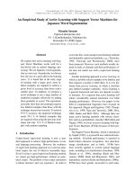
An insightful picture of this geometric separation is given in Fig. 2.1.

Fig. 2.1 The positive and negative
samples, denoted by squares and
circles, respectively. The decision
hyperplane between the two corresponding separable subsets is H.

CuuDuongThanCong.com

H
{x|w⋅x-b<0}

{x|w⋅x-b>0}


10

2 Support Vector Learning and Optimization

It is further resorted to a stronger statement for linear separability, where the
positive and negative samples lie behind a corresponding supporting hyperplane.
Proposition 2.3. [Bosch and Smith, 1998] Two subsets of n-dimensional samples
are linearly separable iff there exist w ∈ Rn and b ∈ R such that, for every sample
i = 1, 2, ..., m:
w · xi − b ≥ 1, yi = 1
w · xi − b ≤ −1, yi = −1

(2.4)

An example for the stronger separation concept is given in Fig. 2.2.

Fig. 2.2 The decision and supporting hyperplanes for the linearly
separable subsets. The separating
hyperplane H is the one that lies in
the middle of the two parallel supporting hyperplanes H1 , H2 for the
two classes. The support vectors are
circled.

H2

H

H1

{x|w⋅x-b=-1}

{x|w⋅x-b=1}

Proof. (we provide a detailed version – as in [Stoean, 2008] – for a gentler flow of
the connections between the different conceptual statements)
Suppose there exist w and b such that the two inequalities hold.
The subsets given by yi = 1 and yi = −1, respectively, are linearly separable since
all positive samples lie on one side of the hyperplane given by
w · x − b = 0,
from:
w · xi − b ≥ 1 > 0 for yi = 1,
and simultaneously:

w · xi − b ≤ −1 < 0 for yi = −1,
so all negative samples lie on the other side of this hyperplane.
Now, conversely, suppose the two subsets are linearly separable. Then, there exist
w ∈ Rn and b ∈ R such that, for i = 1, 2, ..., m:

CuuDuongThanCong.com


2.3 Support Vector Machines with Linear Learning

w · xi − b > 0, yi = 1
w · xi − b ≤ 0, yi = −1
Since:
min {w · xi |yi = 1} > max {w · xi |yi = −1} ,
let us set:
p = min {w · xi |yi = 1} − max{w · xi |yi = −1}
and make:
w =

2
w
p

and
b = 1p (min {w · xi |yi = 1} + max{w · xi |yi = −1})
Then:
min w · xi |yi = 1 =
2
min {w · xi |yi = 1}
p

1
= (min {w · xi |yi = 1} + max{w · xi |yi = −1} +
p
min {w · xi |yi = 1} − max{w · xi |yi = −1})
1
= (min {w · xi |yi = 1} + max{w · xi |yi = −1} + p)
p
= b +1
=

and
max w · xi |yi = −1 =
2
max {w · xi |yi = −1}
p
1
= (min {w · xi |yi = 1} + max{w · xi |yi = −1} − p)
p
= b −1

=

Consequently, there exist w ∈ Rn and b ∈ R such that:
w · xi ≥ b + 1 ⇒ w · xi − b ≥ 1 when yi = 1
and w · xi ≤ b − 1 ⇒ w · xi − b ≤ −1 when yi = −1

CuuDuongThanCong.com

11

12

2 Support Vector Learning and Optimization

Definition 2.2. The support vectors are the training samples for which either the
first or the second line of (2.4) holds with the equality sign.
In other words, the support vectors are the data samples that lie closest to the
decision surface. Their removal would change the found solution. The supporting
hyperplanes are those denoted by the two lines in (2.4), if equalities are stated instead.
Following the geometrical separation statement (2.4), SVMs hence have to determine the optimal values for the coefficients w and b of the decision hyperplane that
linearly partitions the training data. In a more succinct formulation, from (2.4), the
optimal w and b must then satisfy for every i = 1, 2, ..., m:
yi (w · xi − b) − 1 ≥ 0

(2.5)

In addition, according to the SRM principle (Proposition 2.1), separation must be
performed with a high generalization capacity. In order to also address this point, in
the next lines, we will first calculate the margin of separation between classes.
The distance from one random sample z to the separating hyperplane is given by:
|w · z − b|
.
w

(2.6)

Let us subsequently compute the same distance from the samples zi that lie closest to the separating hyperplane on either side of it (the support vectors, see Fig.
2.2). Since zi are situated closest to the decision hyperplane, it results that either
zi ∈ H 1 or zi ∈ H 2 (according to Def. 2.2) and thus |w · zi − b| = 1, for all i.

Hence:
1
|w · zi − b|
=
for all i = 1, 2, ..., m.
w
w

(2.7)

Then, the margin of separation becomes equal to [Vapnik, 2003]:
2
.
w

(2.8)

Proposition 2.4. [Vapnik, 1995b]
Let r be the radius of the smallest ball
Br (a) = {x ∈ Rn | x − a < r} , a ∈ Rn
containing the samples x1 , ..., xm and let
fw,b = sgn(w · x − b)
be the hyperplane decision functions.
Then the set fw,b | w ≤ A has a VC-dimension h (as from Definition 2.1) satisfying

CuuDuongThanCong.com