State and non - state wage differentials in VN

THE ECONOMICS UNIVERSITY
HOCHIMINH CITY
VIETNAM

INSTITUTE OF SOCIAL STUDIES
THE HAGUE
THE NETHERLANDS

VIETNAM- THE NETHERLANDS PROJECT ON DEVELOPMENT ECONOMICS

STATE AND NON-STATE WAGE
DIFFERENTIALS IN VIETNA.M

Supervisor NGUYEN VAN NGAI
Student
TRAN DUONG CHIEN TRANG

Hochiminh City, December 2003


ACKNOWLEDGEMENT

I thank Dutch government for financial supports and Institute of Social Science (ISS),
The Hague for academic program during two-years period of my study.

I am really grateful to my supervisor, Dr. Nguyen Van Ngai for his advices and
comments through all stages of thesis making. I also owe Dr Youdi Schipper and Mr.
Michael Palmer a special thank for all their help during the time of thesis proposal. I
thank Mr. Jeff Collins for English correction and Mr. Truong Dang Thuy and Mr.
Phung Thanh Binh for their comments.

I also want to show my gratitude to all lecturers for providing me academic knowledge
background and to the project staff, Ms. Dinh Thi Anh Nguyet and Ms. Dang Kim Chi,
for their help during the courses.

ii


ACKNOWLEDGEMENT

I thank Dutch government for financial supports and Institute of Social Science (ISS),
The Hague for academic program during two-years period of my study.

I am really grateful to my supervisor, Dr. Nguyen Van Ngai for his advices and
comments through all stages of thesis making. I also owe Dr Youdi Schipper and Mr.
Michael Palmer a special thank for all their help during the time of thesis proposal. I
thank Mr. Jeff Collins for English correction and Mr. Truong Dang Thuy and Mr.
Phung Thanh Binh for their comments.

I also want to show my gratitude to all lecturers for providing me academic knowledge
background and to the project staff, Ms. Dinh Thi Anh Nguyet and Ms. Dang Kim Chi,
for their help during the courses.

11


ABBREVIATIONS

·CWE

Corrected Wage Equation

DPE

Domestic Private Enterprises

FIE

Foreign Investment Enterprises

GDP

Gross Domestic Product

GSO

General Statistical Office

IMR

Inverse Mill's ratio

ISD

Index of Sector Discrimination

LSE

Likelihood Selection Equation

MLA

Maximum Likelihood Approaches

MLE

Maximum Likelihood Estimation

NPV

Net Present Value

OLS

Original Least Squared regression

SOE

. State-owned Enterprises

UCE

Urban Collective Enterprises

VLSS

Vietnam Living Standards Survey

WB

World Bank

111


ABSTRACT
There is no evidence on the extent of wage differentials between state and non-state
sector in Vietnam. The main objection of this research is to examine the wage
differentials between SOE versus DPE and SOE versus FIE, and to find source of the
differentials. For those purpose, corrected Mincer earnings equations of sectors, which
are the Mincer earnings equations corrected selection bias by Heckman Two-Step
method, must be compared by using the Oaxaca-Blinder Decomposition method. The
data sample of VLSS 97-98 is applied for estimation process. The results indicated that
there is sector discrimination in wage against state sector, and the difference in wage
settings the source of the sector discrimination. Besides, there was the hesitation of nonstate participation and gender discrimination in both sectors.

IV


CONTENTS
CER TIFICATI0 N ...........................................................................Cio····················v····· i
A CKNOWLE.DGEMENT
ABBREJ!'l"ATIONS
ABSTRA. CT..........

CONTENTS

ii

oooooooooooooooooooooooooooooooooooooooooooooooooooooooooooooooooooooooooqooooooooooooooooooooooooo

oooooooooooooooooooooooooooooooooooooooooooooooooooooooooooo;,ooooooooooooooooooooollooooooetoooooooooooooooooo

oooe . . . . . . . OOOitO • • • • • • • • • • • • • • • • • • It • • • • • • • • 0

000 0 0000 • • 0000 • • • • • 0 • • • 0 0 • • • • • • • • • • • • • • •

ooo. 0

iii
iv

••••••••••••••• 0. 0 0 •••

oooooooooooooooooooooooooooooooooooooooo•oooooooooooooooooooooooooooooooooooooooooooooooooooooooctooooooooooooo•••••••••••

LIST OF TABLES..••.••.••.•...••.•.•...........•...••..•...•.........•..

V

vi

eo ••••••••••••••••••••••••••••••••••••••••••••••••••••

LIST OF FIGURES ···················eo·················o·······························································.,····· vi
CHAPTER 1:INTRODUCTION•..•..•
1
1.1. Problem statement and the objective of the research ........ ~ .................................... 1
1.2. Research question ....................................................................................................... 2
1.3. Methodology and dataset ........................................................................................... 3
1.4. Structure of the thesis ................................................................................................. 3

o ••••••••••• e •••••••••••••••••••• e . . . . . . . . . . . . . . . . . . . . . . . . . . . . . . . . . . . . . . . . . . . . . . . . .

CHAPTER 2: LITERATURE & EMPIRICAL REVIEW ........•........................................... 5
2.1. Definitions ................................................................................................................... 5
2.2. Theoretical Review .................................................................................................... 7
2.3. Empirical studies ...................................................................................................... 18
2.4. Vietnam labor market overview: ............................................................................ 21
CHAPTER 3: MODEL SPECIFICATION AND DATABASE .......................................... 24
3.1. Corrected Wages Model (CWE) ............................................................................. 24
3.2. Likelihood Selection Model (LSE): ....................................................................... 27
3.3 Calculation ofthe inverse Mill's ratio (IMR): ....................................................... 31
-.. - ·.
3.4. Database ................................................................................................................................ 31
CHAPTER 4: STATE AND NON-STATE WAGE DIFFERENTIALS IN WETNAM....... 34
4.1. Descriptive Analysis ................................................................................................ 34
4.2. Econometric Analysis .............................................................................................. 57
4.3. Comparison with other researches ......................................................................... 79
CHAPTER 5: CONCLUSIONS AND POLICY IMPLICATION........................................ 82
5 .1. Conclusion ................................................................................................................. 82
5.2. Policy implication ................................................................................. ~ ................... 84
5.3. Further researches ..................................................................................................... 85
APPENDIX..•... ., .•.......•.......•...........•...............................................•................................. 8 7
BIBLIOGRA.PHY••.......••.........................................................................................

o ••••••••

94

v

LIST OF TABLES
Table 2.1: Identification of the earnings and sector choice equations .................................................... 20
Table 3.1. Specification of the corrected wages model............................................................................ 27
Table 3.2. Specification of the Likelihood Selection Model (LSE) .......................................................... 30
Table 4.1. Types of data and levels ofmeasurement ............................................................................... 35
Table 4.2: Descriptive statistics ............................................................................................................... 36
Table 4.2: Descriptive statistics (continue) ............................................................................................. 37
Table 4.3. Statistic Analysis of Wage ....................................................................................................... 39
Table 4.4. Statistic Analysis ofAge.......................................................................................................... 40
Table 4.5. Statistic Analysis of Experience .............................................................................................. 41
Table 4.6. Education and wage rate ................................................................... :.................................... 42
Table 4. 7. ANO VA results for wage and education relationship ............................................................. 44
Table 4.8. Experience and Wage Rate ..................................................................................................... 44
Table 4.9. ANOVA results for wage and experience relationship ........................................................... 46
Table 4.1 0. Gender and wage rate ........................................................................................................... 4 6
Table 4.11 t-testfor wage difference between gender group ................................................................... 47
Table 4.12. Location and Wage Rate ....................................................................................................... 48
Table 4.13 t-testfor wage difference between residua/location groups ................................................. 49
Table 4.14 Regions and Wage Rate ......................................................................................................... 4 9
Table 4.15. ANO VA results for wage and regions relationship ............................................................... 51
Table 4.16. Age and Wage Rate ............................................................................................................... 51
Table 4.17. ANOVA results for wage and age relationship ..................................................................... 52
Table 4.18.a Pearson correlation coefficients among variables for SOE ............................................... 54
Table 4.18. b Pearson correlation coefficients among variables for DPE ............................................... 55
Table 4.18.c Pearson correlation coefficient!/among variables for FIE ................................................. 56
Table 4.19.a: Heckman model for the logarithm of hourly wage ofSOE, DPE, and FIE in 1998 .......... 57
Table 4.19.b: Heckman mode/for the logarithm of hourly wage ofSOE, DPE, and FIE in 1998 (cont) 58
Table 4.20. Wald test offunctional specification ..................................................................................... 59
T~ble 4.20.1 The significance and sign of difference in size of the coefficients ...................................... 59

Table 4.21: The likelihood ratio test for the likelihood selection models ................................................ 61
Table 4.22: Expected Log Hourly Wages by Sector of Employment, Vietnam 1997-98 .......................... 67

vi


Table 4.23: Decomposition ofstate and non-state wage differentials in Vietnam 1997-98 .................... 73
Table 4.23: Decomposition ofstate and non-state wage differentials Vietnam 1997-98 (cant) .............. 74
Table 6.1 Pooling Regression .................................................................................................................. 93

vii


LIST OF FIGURES
Figure 2.1. Employment choice ............................................................................................. 8
Figure 4.1. Education and Wage rate ................................................................................... 44
Figure 4.2. Years ofExperience and Log wage rate ............................................................. 46
Figure 4.3. Gender and Wage rate ........................................................................................ 48
Figure 4.4. Wage rate and Location groups ......................................................................... 49
Figure 4.5. Wage differentials between regions .................................................................... 51
Figure 4.6. The relationship between wage and age ............................................................. 53
Figure 4. 7. Effects of education attainments on (log) hourly wages ..................................... 69
Figure 4.8. Gender wage differentials among sectors .......................................................... 71
Figure 4.9. Effects of seniority on (log) hourly wages.......................................................... 71
Figure 4.1 0. Effects of location to expected wages ................................................ :.............. 72
Figure 4.11. Effects of regions to expected wages ................................................................ 73

viii

CHAPTER l:INTRODUCTION
1.1. Problem statement and the objective of the research
Since 1986, Vietnam has adopted the doi moi (renovation) policy to transform from the
centrally planned economy to a socialist oriented market economy. The reform involved
expanding the private sector and opening up the economy. These changes have
contributed impressive results to economic growth. During the period 1993-1997, GDP
was increased at a rate of approximately 9% per year, of which the share of the nonstate sector in GDP was about 60 per cent (Belser 2000 and GSO 2000).

Matters exist where "over-sized" state-owned enterprises (SOE) have become a
significant burden to the government budget. SOE showed a decreasing trend
contribution to the growth of GDP from 11.4 percent to 9.7 percent in 1996 and 1997
respectively but wages and expenditure increased at the rate of 6.2 percent and 6.9
percent. At the same time the number of SOE wage employment increased from 15.48
percent to 16.45 percent in the period of 1992-93 to 1997-98 (World Bank 1999 and
Bales 2000).

There are a difference between the state sector and non-state sector in Vietnam in wage
structure and employment practices. A non-market process sets wages for SOE. A base
salary for each education 1evel i s s et and incremented every three years according to
seniority. There are differentials according to the position occupied. Performance seems
irrelevant iii promotions. SOE employees have lifetime labor contracts and almost 100
percent are union members; however, they are not allowed collective bargaining or the
rjght to strike. Conversely in the non-state sector, which comprises domestic private
enterprises (DPE) and foreign investment enterprises (FIE), wages are set according to
the position occupied and collective bargaining. Performance is important in the

1

consideration of promotion. Employees in the non-state sector have an open-ended labor
contract, which can be canceled following a notice period.

There were a number of studies into the wage differentials between public and private
sector (Gunderson 1979, Gyourko and Tracy 1988, Hartog and Oosterbeck 1993, Terrell
1993, Bedi 1998, Tansel 1999, and Zhao 2001). The public sector typically comprises
government administration and SOE, and the private sector covers those employees
included in social security and health schemes (Tansel 1999 and Zhao 2001). But such
study has not been found in Vietnam. The goal of such study is to investigate the wage
differentials between the state sector and the non-state sector in Vietnam. The state
sector has a surplus of labor and has constraints to voluntarily lay-off workers and the
number of wage employment in the non-state sector showed a decreasing trend. These
indicators may lead to the conclusion that the wages of workers in SOE are higher than
those of DPE and of FIE. The results of this research will provide policymakers with a
clearer idea of whether or not the state worker earned the premium wage, and where are
sources of the wage differentials between state and non-state sector. From those
findings, suitable policies could be applied to adjust the SOE wage settings and
employment practices for increasing SOE performance and decreasing SOE fiscal
problems.

1.2. Research question

This research aims to investigate the wage differentials between state sector and nonstate sector in Vietnam. To further this investigation the following research questions
are proposed:
1. "Are the earnings of SOE workers higher than the earnings of DPE and of FIE
workers in Vietnam?"
2. and "where are sources of the net earnings differentials between SOE versus
DPE and FIE?"

2

1.3. Methodology and dataset
The public sector is the state sector with government administration and the private
sector is non-state sector. Government administrative organizations were excluded from
the research because their objective is broader than profit maximization of an enterprise
(Borjas 1996). The comparison group for research is based on an enterprise category.

In order to answer the first question, the method of comparing sectoral Mincer earnings
equations is applied .. However?. the estimates of these Mincer earnings equations are
inconsistent because of selection bias so that the Heckman Two-Step Method must be
applied to specify the corrected Mincer earnings equations. The Oaxaca-Blinder
Decomposition method will be used to answer the second question. The Oaxaca-Blinder
Decomposition method will decompose the net wage differentials into four components
included constant terms, endowments, coefficients, and selection bias. Econometric
analysis helps to find the effects of various determinants on wage. Descriptive statistics
are also used to clarify the content of the dataset. Regression is different to descriptive
statistics.

The data used for the study were derived from the Vietnam Living Standard Survey in
1997/1998 (VLSS 97-98). This research uses cross section data of interviewees of the
survey. Because the research focuses on the labor market, the data sample will be
restricted to individuals aged 15-65"'",;"'
~·
1.4. Structure of the thesis

The research is organized as follows.

Chapter 1 provides basic information and a background to the research.

3


Chapter 2 will provide the I iterature on i ndividuall abor supply, human capital, labor
market discrimination, institutional approach to labor market, the Heckman's Two-Step
Method, and the Oaxaca-Blinder Decomposition Method, which theoretically supports
the answer to the question in literature section. An empirical studies' review follows.
Lastly the current situation of wage employment and wage differentials among sectors
in Vietnam will be demonstrated.

Chapter 3 will specify the model and database used for this study.

Chapter 4 will present descriptive statistics oft he dataset, the estimation models and
their results. The latter section will focus on the results of the analysis in comparison
with previous studies.

Chapter 5 draws some conclusions and provides for policy implementation.

4


CHAPTER 2: LITERATURE & EMPIRICAL REVIEW

The chapter first provides some definitions related to this study. The theoretical review
then investigate the choice between two sectors as these choices relate to the wage
differentials among employees, and the source of these wage differentials. The chapter
continues with empirical studies. These will involve research of public and private wage
differentials in Turkey and China whose methodology approximates this study. Finally,
the chapter will review the Vietnam labor market and the differences between the state
and non- state sectors.

2.1. Definitions

The worker's earnings are the sum of wages, bonus, and other compensations in kind
collected per working hour. There is no distinction between earnings and wages.

The state sector is defined as the state-owned enterprises (SOE) and the non-state sector
as the foreign investment enterprises (FIE) and the domestic private enterprises (DPE).

The FIE include 100 percent foreign owned enterprises and joint venture enterprises.
The DPE include cooperatives, private enterprises, small household enterprises, and
mixed enterprises (GSO 2000).

Mincer's Earning Equation implies wage determinants under age-earnmgs profiles
while the corrected wage equations (CWE) are considered as the Mincer's earning
equation under corrected selection bias.

5


The likelihood selection equation (LSE) is the likelihood equation of multinomial sector
choice probit equation, which explains the probability of sector participation of an
individual.

The Ordinary Least Squares method (OLS) is the method to construct the sample
regression function that is basis to estimate the population regression function (Gujarati
1995).

Selection bias in the thesis is

t~e

problem in OLS estimation of a Mincer earnings

equation. The problem emanates from two sources. Firstly, there is self-selection among
individuals when they participate in the labor market and are employed into sectors.
Sample data collected is not stochastic. Secondly, wage data is not available for nonworkers or of wage reservation hence the Mincer's earnings equation becomes a
censored regression model. The bias leads the OLS estimation of the Mincer earnings
equation to provide inconsistent co-efficient estimates.

Inverse MilT's Ratio (IMR) or selection term, which is calculated from the estimated
probability value of the LSE, is used for correcting inconsistent estimates of parameters
in OLS regression of the Mincer earnings equation in the Heckman Two-Step Method.
The IMR represents the probability of sector participation in the sectoral CWE (Pindyck
and Rubinfeld 1998).

There is a distinction between Maximum-Likelihood Approach (MLA) and Maximum
Likelihood Estimation (MLE). MLA is the application of the maximum-likelihood
approach to estimate linear models and non-linear models (Pindyck and Rubinfeld
t"998). MLE is an alternative method of selection bias correction (Brendt 1991 ).

6


2.2. Theoretical Review
The

theoretica~

review will investigate the theory of individual labor supply to explain

the decision of whether to work or not and in which sector to participate, the theory of
traditional ·human capital and labor market discrimination describing why there are
wage differentials among workers.

2.2.1. The theory of individual labor supply
The theory of individual labor supply explains how an individual selects employment.
In essence, the theory of individual labor supply is an application of the theory of
consumer behavior. It is assumed that an individual who is constrained by time and
budget can afford consumer goods. An individual should allocate a number of hours
available between leisure activities and the labor market, and have available non-labor
income (property income, lottery prizes, and remittances) and 1abor income (equal to
hourly wage rate and total working hours) (Berndt 1991, and Borjas 1996). Income can
be increased by sacrificing hours of leisure for additional hours of work. The budget
line presents the boundary of individual opportunity set between hours of leisure and
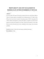
income (or consumption). EL, EM, and EH respectively in Figure 2.1 illustrate budget
lines at each hourly wage rate. OV describes non-labor income, OT is available total
number of hours, and hours wage rates included W reservation, W low, W high are slopes of
budget lines EL, EM, EH respectively. It is also possible to choose a combination of
consumption and hours of leisure that maximizes utility. The indifference curve
represents a particular level of individual satisfaction or an indifferent choice between
consumption and hours of leisure. The UO, U1, U2 curve in Figure 2.1 illustrates levels
of individual utility or satisfaction. The U2 curve gives the highest level of individual
utility, and U0 the lowest level.

7


Consumption ($)

H

·,.

·,.

M

·,.

·,.·,.

·,.·,.

·,.

·,.

·,..·,.

·,.

/

Slope -W high

·,.

~
·,..

Slope -Wiow

·:-...

v ............................................................................................... . !
~

0

·-·-·-·-·-·-. ----- u2

T
Hours of
Leisure

Figure 2.1 employment choices
Source: To work or not to work (Borjas 1996 p.31) and Consumer Behavior (Pindyck and
Rubinfeld 1998 p.57-78)

Point E where the indifference curve U0 touches the budget line EL with hours wage
rate of

Wreservation

is the point at which an individual decides to work or not to work.

Here the hours wage rate

Wreservation

is called the reservation wage. An individual will

decide to enter the labor market when the offered wage is higher than the reservation
wage. The reservation wage is affected by factors including hours ofleisure, non-labor
income, and the prices of consumer goods (Berndt 1991, and Borjas 1996). Similarly,
with the hours wage rate Whigh higher than W1ow, a worker who has a budget line EH
reaches the indifference curve U2 higher than U 1 of another worker who has a budget
line EM. The worker will decide to participate in a particular sector whenever they
perceive the wage in this sector is higher than the wage in the other sectors, ceteris
8


paribus. Ceteris paribus is the notion of exogenous factors. However, workers are
different so the reservation wage will vary from worker to the worker. (Borjas 1996).

2.2.2. The theory of neoclassical human capital
The neoclassical human capital theory best explains wage determinants among workers
because the theory explains why there should be wage differences for different workers
in a perfect labor market (Fine 1998). Accordingly, workers vary in ability and acquired
skills or human capital. Human capital can be gained through education, training, and
work experience (Borjas 1996, and Fine 1998). The theory assumes that the individual
present value of age-earnings profiles is
NPV = -C-

c

c

-

(1 + r)

(1 + r

Y

-A -

c

=-I
t=O

c

(1+r)

t

+

f

w

w

(1 + r Y (1 + r Y+I

Costs of attending school/ college

NPV

+

+

w
(1 + r y+

2

w

+A +

or

(1 + r )"

The return to schooling

I

t=i+I(1+r)

where NPV is Net Present Value of individual age-earnings, n is lifetime and r is the
rate of discount. A student must pay for books, fees, and so on (C) throughout years of
schooling (i) to receive a future wage (W) as the return for schooling throughout a

working life (n-i). The model not only explains how an individual decides how much
schooling to acquire but also indicates the wage gap among workers because of the
education difference. Accordingly, a person self-estimates a rate of discount depended
on the probability of future rewards or on the return for schooling, therefore the future
wage (W) among workers varies according to educational achievements, ceteris paribus.
Even if the rate of discount is similar, there are differences in individual abilities hence
...

the future wage (W) and the wage-schooling locus, which is the salary that employers
are willing to pay for every level of schooling, differs from worker to worker. Similarly,
the theory considers the on-the-job training during working time as human capital

9


investment. The employer when hiring a worker must pay a salary (W) and implicated
on-job-training fees (G) so the employer will pay a salary (W2 = W +G) in the next year:
for the accumulated experience of the worker.

In many empirical studies, the Mincer's earmngs equation 1s considered as the
implications of the human capital model for the age-earnings profile to. explain wage
determinants of workers (Mincer 1974, Berndt 1991, Bmjas 1996). This expressed as
follows:
logW = w(EDU, EXP, EXP

2

,

AGE, OTHER)

(2.1)

where W is earnings, EDU is education, EXP is experience, EXP 2 is a quadratic on
EXP, AGE is age of employees, OTHER are other factors which affect wage
determinants (Borjas 1996). The logarithm of wage is used instead of the actual wage
because logarithms can be used to compare positive numbers. Consider W 1 and W 2 as
the wage oft he worker 1 and 2 respectively, and when the wage difference between
workers is small, the result is:

logW2 -logw; =

W2-~

JY1

o

= Yof1W

(2.2)

so that the difference in logs equals the percentage difference between the two wages.
The EDU is measured by the number of years of schooling. Under the age-earnings
profile, the rate of return on the first year of schooling (r 1) is,
(2.3)
W 1 is earnings after one year of schooling and W 0 is earnings without education (Borjas
1996, Berndt 1991)

From (2.3),

W1

= W0 (1 + r)

(2.4)

10


After EDU years of schooling, incremental earnings are,
(2.5)

If the rate of the return is the same for all levels of schooling, r 1 = r2 = r3 = ... = rx and (1

+ r) approximate eR as well as the multiplicative disturbance term eu appended, the
equation (2.5) will become

logrt: =logffo +rEDU+U

(2.6)

The on-job-training is measured by the working time devoted to training investment,
which is calculated by a multiplication between the proportion of working time saved
for on-job-training (k) and years of working experience (EXP). Unfortunately, data on k
is missing data in all data sources. Further, tJ;le neoclassical theory of human capital
suggested that worker's earnings curve follows parabolic shape over working time
because worker acquires more human capital when young and less that when older
(Borjas 1996). This led Mincer to use two variables for years of working experience
(EXP) and quadratic on EXP (EXP 2) for measuring the value of on-job-training human

capital. The age of worker (AGE) should be added into the wage equation because of
the effect of overtaking age (Borjas 1996). One important assumption of the
neoclassical paradigm is a perfect competitive market. Notwithstanding this assumption
the worker generally meets an imperfect labor market. As a result Mincer's earnings
equation requires additional variables (OTHER).

2.2.3. The theory of labor market discrimination
In the imperfect labor market, the worker is not only differs from other workers in
human capital but also is discriminated by his individual characteristics. The theory of
labor market discrimination demonstrated that wage differentials among workers
emanated from taste discrimination including race and gender (Borjas 1996). For
instance, a white employee may not like to work for a black employer and with black

11


colleagues. An employer could take into account the race and the gender of the
applicant, and the consumer may discriminate about the gender and race of the seller.
The employer could be willing to pay a wage (W) for a worker but could vary the wage
for a black worker or for a female worker to W 1 x ( 1+d), where d is the discrimination
parameter. So the recruitment decision is based on a comparison of W and W 1 x ( 1+d),
employer hire only for black workers or for females workers if W 1 x ( 1+d) < W and hire
only white workers or male workers if W 1 x (1 +d)> W. The Mincer earnings equation
then explains the wage differentials among workers should take into account gender
(SEX) and race (RACE) variables as follows (Fine 1998):

logW = W(EDU,EXP,EXS,AGE,SEX,RACE)

(2.7)

2.2.4. Institutional approaches to the labor market
Wage determinants exist among workers, but decision of labor participation and of
sector participation respectively based on the level of reservation wage and sectoral
wage. In answer to the question of what is the source of wage differentials between the
state and the non-state sector, institutional approaches to the labor market explicitly
explain the differentials as political (Fine 1998). Accordingly, the state sector is
suspected to have a higher than competitive wage because the state sector is supported
by government. If the non-state company pays more than market wage, they could
reduce profits or get the loss. These results will encourage the fim1s to no longer
overpay. While the bad financial situation resulting from this behavior in state firms is
simply passed on to taxpayers. Unfortunately, taxpayers have little opportunity to look
after what their representatives are using the budgets from tax. Moreover, the state has a
political incentive to overpay employees. The vote and the potential political force of
state workers are reasons to overpay the state employees for their cooperation and
political support. The differentials could also emanate from institution arrangements in
communist countries as reported by Borjas (Borjas 1996). In the communist countries,
the political institution is built on single communist party. The communist party gathers

12


their fundamental force from public worker so that public worker should earn an
overpaid wage by political target. The worker could perceive the sector difference from
wage and employment settings as well as the non-pecuniary aspects (Tansel 1999 and
Zhao2001).

2.2.5. Estimation Methods:
In practical terms, the state and the non-state wage differentials can b e c omputed b y
OLS regression in at least in 2 procedures. One procedure uses a dummy sector variable
in a statistical Mincer's earnings function. The other procedure aims to separate the

'

sample into state and non-state workers and to estimate separate Mincer earnings
equations with both intercept and slope coefficients differing, then the wage
differentials will be estimated throughout decomposed components of the wage
equations by the Oaxaca-Blinder Decomposition method (Oaxaca 1973, Blinder 1974,
Berndt 1991). However, workers who have either a very 1ow market w age or a v ery
high reservation wage will not work. Furthermore workers may participate in the state
sectorbecausethewage in SOE is higher than the other sources (Borjas· 1996). This
means there is a self-selection among workers hence the sample of workers is not a
random sample. Besides, wage data is not available fort hen on-worker. The missing
data problem is covered as a dependent variable in Mincer earnings equation. So, both
of these errors are called a sample-selection bias or self- selection bias (Heckman 1979).
For example, the motivation of Mincer earnings equation (2. 7) comes from the fact that
·it observes earnings for individuals who are working but does not observe earnings for
individuals who are not working. The equation (2.7) can be rewritten as

log W = {JX + u (2 .8)
where X is vector of explanatory variables

~

is a vector of unknown parameters of these

variables and u is the error term. A vector of estimated inconsistent parameters

~

will

result if the estimate equation (2.8) includes observations where individuals have a
wage. However, individuals only participate in work whenever the wage of the work
13


(W) is higher than reservation wage (Wr)_ (Bmjas 1996). The reservation wage

1S

assumed as

togw; = rXr + u'

(2.9)

where Xr is a vector of variables, which determine the participation decision of
individuals as compared to X's vector determination W; y is a vector of parameters of
Xr; and u' is an error term. As a result of (W > Wr),

(2.10.a) or

j3X- rXr + v > 0
where

v = (u - u,).

(2.10.b)

The cov(u, u,) will not equal zero in order for the result of ~X with

the sample of employees to lead to biased estimates of
sector choice

shoul~

~

for whole population. Thus,

be employed in the research of wage differentials.

There are two methods that can be applied to correct the selection bias of the Mincer
earnings equation including Heckman's Two-Step Method and Maximum Likelihood
Estim~tion

Methpd (MLE) (Pindyck and R1,1bi~f~ld 1998, Yun 1999).

2.2.5.1. The Heckman's Two-Step Estimation Method

In the Heckman's Two-Step Method, an individual decide to work if their expected
wage is higher than their reservation wage, and a worker decide to join a sector by
perceiving the net c}iffer~ntials in wage and non-wage compensation in each of these
sectors. The taste
~ontribute

~nd

preference of employees, human capital, other characteristics

to determine the sector selectivity (Lewis 1996). Thus, the probability (Pj)

that an individual choic.e in alternative j sector is assumed as:

14


(2.11)

wh~re

n is a total of sector choices, Z is a vector of explanatory variables affecting

sector choice, and a is a vector of unknown parameters of the alternative j. Equation
(2.11) is a

sta~d1:1rd

probit equation, and its parameters (a) can be estimated by

maximizing the LSE Pj (or its logarithm) using the

en~ire

sample of workers and non-

workers in the first step of the m¥thpd. The estimates Pj parameters are then used to
compute estimates of the IMR (A.) as follows:

Here,

$ is the Standard Normal Density Function, and <I> is the Standard Nonnal

Distribution Function. In step 2 of the method, the estimated IMR (A.j) will be appended
as an additional regressor (called selection term) to the sectoral Mincer's model to
obtain the sectoral CWE. Thus, the model is developed as follows:

logW = W(EDU,EPX,EXS,AGE,SEX,RACE,/L)

(2.13)

By using an OLS estimation of the model (2.13) with data on sector workers only obtain
consistent estimates of the parameters can be obtained (Berndt 1991 and Tansel1999).

After the selection bias-corrected parameter and the selection term of sectors are
estimated, the Oaxaca-Blinder decomposition mythod will be applied to decomposing
wage differentials between sectors (Oaxaca 1973, Blinder 1974, Berndt 1991). The
method assumes that in the absence of differentials the estimated effects of employees'
endowments on earnings are identical for each sector j. Let j=O represent the non-state
sector andj=1 represent state sector in model (2.14):

15


log~ -logWo = (f3ot- f3oo)+ ..Bo (:XI- Xo )+ (,81- f3o )XJ +(.n-1 ~ -7Z"oAo )(2.14.b) or
logYJ?; -logf¥o =(Poi- f3oo)+0.5(f31 + f3o)('xi -xo)+o.5(f31- Po

XXI +Xo)+(7r~~ -1l"oAu)(2.14.c)

where over-bar denotes the mean of variables. The mean of log wage differentials is
decomposed into the four components in the right of the equation. The first component

is the difference in constant terms. This is often interpreted as the premium from being
· in a given sector (Terrell 1993). The second component explains the difference in
employees' endowments, and the third component is due to the market returns to the
endowments. The final component reveals the difference in the selection bias (A= n.A).
The first and the third components constitute the total structure differential that answers
to the first research question whether the state earns the premium. Take an example of
the equation (2.14.c); the total structure differential (Dg) can be re-written as follows:

Dg = 0.5[(f3ot + fJ1 (XI + Xo )) -

The term

(..Boi + ,81(XI+ Xo))

(Poo +Po (XI + Xo ))]

(2.15)

is considered as the hypothetical earnings (in logarithm)

of workers in both sectors when they work with their own productivity but earn
according to the CWE of state sector. While the term

(Poo + flo(X 1 + Xo))

is the

hypothetical earnings (in logarithm) of all workers according to the CWE of non-state
sector. So the sector d iscrimiJ.?.ation is the total structure differentials ( Dg), which is
computed by the average difference between the hypothetical earnings according .to the

CWE of state sector and those of non-state sector.

16