Thời gian thực - hệ thống P6
Bạn đang xem bản rút gọn của tài liệu. Xem và tải ngay bản đầy đủ của tài liệu tại đây (355.31 KB, 39 trang )
CHAPTER 6
REAL-TIME LOGIC,
GRAPH-THEORETIC ANALYSIS,
AND MODECHART
A real-time system can be specified in one of two ways. The first is to structurally
and functionally describe the system by specifying its mechanical, electrical, and
electronic components. This type of specification shows how the components of the
system work as well as their functions and operations. The second is to describe
the behavior of the system in response to actions and events. Here, the specification
tells sequences of events allowed by the system. For instance, a structural-functional
specification of the real-time anti-lock braking system in an automobile describes
the braking system components and sensors, how they are interconnected, and how
the actions of each component affects the other. This specification shows, for ex-
ample, how to connect the wheel sensors to the central decision-making computer
that controls the brake mechanism.
On the other hand, a behavioral specification shows only the response of each
braking system component in response to an internal or external event, but does not
describe how one can build such a system. For instance, this specification shows that
when the wheel sensors detect wet road conditions, the decision-making computer
will instruct the brake mechanism to pump the brakes at a higher frequency within
100 ms. Since we are interested in the timing properties of the system, a behavioral
specification without the complexity of the structural specification often suffices for
verifying the satisfaction of many timing constraints. Furthermore, to reduce specifi-
cation and analysis complexity, we restrict the specification language to handle only
timing relations. This is a departure from techniques that employ specification lan-
guages capable of describing logical as well as timing relations, such as real-time
CTL.
148
Real-Time Systems: Scheduling, Analysis, and Verification. Albert M. K. Cheng
Copyright
2002 John Wiley & Sons, Inc.
ISBN: 0-471-18406-3
EVENT-ACTION MODEL
149
6.1 SPECIFICATION AND SAFETY ASSERTIONS
To show that a system or program meets certain safety properties, we can relate
the specification of the system to the safety assertion representing the desired safety
properties. This assumes that the actual implementation of the system is faithful to
the specification. Note that even though a behavioral specification does not show how
one can build the specified system, one can certainly show that the implemented sys-
tem, built from the structural-functional specification, satisfies the behavioral speci-
fication.
One of the following three cases may result from the analysis relating the specifi-
cation and the safety assertion:
1. The safety assertion is a theorem derivable from the specification, thus the
system is safe with respect to the behavior denoted by the safety assertion.
2. The safety assertion is unsatisfiable with respect to the specification, so the sys-
tem is inherently unsafe since the specification will cause the safety assertion
to be violated.
3. The negation of the safety assertion is satisfiable under certain conditions,
meaning that additional constraints must be added to the system to ensure its
safety.
The specification and the safety assertion can be written in one of several real-
time specification languages. The choice of language would in turn determine the
algorithms that can be used for the analysis and verification. We begin the study with
the event-action model and a first-order logic called real-time logic (RTL) [Jahanian
and Mok, 1986].
6.2 EVENT-ACTION MODEL
The event-action model [Heninger, 1980; Jahanian and Mok, 1986] captures the data
dependency and temporal ordering of computational actions that must be taken in
response to events in a real-time application. There are four basic concepts.
1. An action is a schedulable unit of work and can be primitive or composite. A
primitive action is atomic in that it cannot or does not need to be broken into
subactions for the purpose of analysis. It consumes a bounded amount of time.
A composite action is a partial ordering of primitive actions or other composite
actions. The same action may appear more than once in a composite action.
Recursive actions and circular chains of actions where an action is a subaction
of its predecessor in the chain are not allowed.
The notation A;B indicates that the sequential execution of action A is fol-
lowed by action B. For example, TRAIN-APPROACH;DOWN-GATE means
that the train first approaches the railroad crossing sensor, then the gate moves
150
REAL-TIME LOGIC, GRAPH-THEORETIC ANALYSIS, AND MODECHART
down. The notation AB indicates the parallel execution of action A and action
B. For example, DOWN-GATERING-BELL means that the moving-down of
the gate and the ringing of the alerting bell happen simultaneously.
2. A state predicate is an assertion about the state of the specified system. For
example, GATE-IS-DOWN is true if the gate is in the down position.
3. An event is a temporal marker for indicating a point in time that is significant
in describing the system behavior. There are four classes of events:
(a) An external event is caused by actions outside the specified system.
For example, APPLY-BRAKE is an external event which means the
pressing of the brake pedal by the drive or operator.
(b) A start event marks the beginning of an action, for example, the start
of the DOWN-GATE action.
(c) A stop event marks the end of an action, for example, the end of the
DOWN-GATE action.
(d) A transition event marks the change in a certain attribute of the system
state. For example, GATE-IS-DOWN becomes true when the gate is
moved to the down position.
4. A timing constraint is an assertion about the absolute timing of system events.
6.3 REAL-TIME LOGIC
The motivation for introducing real-time logic [Jahanian and Mok, 1986] is that the
specifications written in the event-action model cannot be easily to manipulated by
a computer. RTL is a first-order logic with special features to capture the timing re-
quirements of the specified system while making the specification easy to manipulate
mechanically. RTL was especially attractive because at the time of its introduction,
temporal logic was able to express relative ordering of events or actions [Heninger,
1980; Bernstein and Harter, 1981], but temporal logic has not yet been extended with
the capability of expressing absolute timing characteristics.
For example, conventional temporal logic can specify that an action B follows
another action A such as TRAIN-APPROACH followed by DOWN-GATE, but can-
not specify that DOWN-GATE will occur within a certain time period (say 5 s) after
the occurrence of TRAIN-APPROACH. Furthermore, temporal logic uses an inter-
leaving model of computation to specify concurrency in computer systems, but this
model cannot express true parallelism. For example, temporal logic models two par-
allel actions as if one is followed by the other or vice versa, so that from an initial
state s
0
there are two paths, corresponding to the two orderings of these actions,
leading to state s
1
.
A scheduler is often an integral part of a real-time system. The correctness of a
real-time system depends on the correctness of its scheduler. Temporal logic, how-
ever, usually assumes the fair scheduling of the specified system’s resources and
events. This is appropriate for non-time-critical systems but certainly is not suffi-
cient for the analysis of real-time systems.
REAL-TIME LOGIC
151
RTL is based on the event-action model, augmented with several features such
as the occurrence function @, which assigns time values to event occurrences.
@(TrainApproach, i) = x means that the ith occurrence of the train approach oc-
curs at time x. There are three types of RTL constants: actions, events, and integers.
Action constants are as defined in the event-action model and capital letters are used
to denote them to distinguish them from variables. A subaction B
i
of a composite
action A is denoted as A.B
i
. Event constants serve as temporal markers and are
classified into: (1) start events indicating the beginning of actions, preceded by ↑;
(2) stop events indicating the end of actions, preceded by ↓; (3) transition events
indicating the change in certain attributes of the system state; and (4) external events,
preceded by .
Example. We now use RTL to specify a simple railroad crossing with one train rail.
From the field measurements and the knowledge about the mechanical characteristics
of the train, train sensor, gate controller, and gate, we obtain the following specifica-
tions. The goal of the gate controller is to ensure that when the train is crossing the
intersection of the road with the rail, no car is on the intersection. In this simplified
version, this is achieved by having the gate in the down position when the train is
crossing.
Specification in English: When the train approaches the train sensor and is detected
by the sensor, a signal is sent to the gate controller to initiate the lowering of the gate
at the railroad crossing.
The gate will be moved to the down position within 30 s from the time when the
train approach is detected by the sensor.
The gate needs at least 15 s to lower itself to the down position.
Safety Assertion in English: If the train needs at least 45 s to travel from the sensor
position to the railroad crossing, and the train crossing is completed within 60 s from
the time the train is detected by the sensor, then we are assured that at the start
of the train crossing the gate has moved to the down position and that the train leaves
the railroad crossing within 45 s from the time the gate has completed moving to the
down position.
We now show the specification and the safety assertion in RTL.
Specification in RTL:
∀x@(TrainApproach, x) ≤ @(↑ Downgate, x) ∧
@(↓ Downgate, x ) ≤ @(TrainApproach, x) + 30
∀y@(↑ Downgate, y) + 15 ≤ @(↓ Downgate, y)
152
REAL-TIME LOGIC, GRAPH-THEORETIC ANALYSIS, AND MODECHART
Safety Assertion in RTL:
∀t∀u@(TrainApproach, t) + 45 ≤ @(Crossing, u) ∧
@(Crossing, u)<@(TrainApproach, t) + 60 →
@(↓ Downgate, t) ≤ @(Crossing, u) ∧
@(Crossing, u) ≤ @(↓ Downgate, t ) + 45
To use existing theorem proving methods [Chang and Lee, 1973] to prove that the
safety assertion (SA) is a theorem derivable from the specification (SP), we further
translate the above into Presburger arithmetic formulas. The following Presburger
arithmetic formulas with uninterpreted functions correspond to the RTL formulas
describing the SP and SA.
Specification in Presburger Arithmetic Formulas:
∀xf(x) ≤ g
1
(x) ∧ g
2
(x) ≤ f (x) + 30
∀yg
1
(y) + 15 ≤ g
2
(y)
Safety Assertion in Presburger Arithmetic Formulas:
∀t∀uf(t ) + 45 ≤ h(u) ∧ h(u)< f (t) + 60 →
g
2
(t) ≤ h(u) ∧ h(u) ≤ g
2
(t) + 45
In these formulas, t, u, x,andy are variables, f , g
1
, g
2
,andh are uninterpreted
integer functions. f corresponds to the occurrence function for event TrainApproach.
g
1
corresponds to the occurrence function for the start of action Downgate. g
2
corre-
sponds to the occurrence function for the end of action Downgate. h corresponds to
the occurrence function for event Crossing.
The problem of determining whether SA follows from SP is in general undecid-
able for the full set of RTL formulas, so not all analysis problems of this type can
be solved. For the subclass of RTL formulas that are decidable, the solutions still
require exponential run time.
Several ways are available to improve the efficiency of the analysis. First, we
can use approximations to yield a simpler set of specification and safety assertions
for analysis. Second, we can focus the analysis on the part of the specification that
is relevant to the validity of the given safety assertions. Third, we can restrict the
specification language so that less general but more efficient analysis procedures can
be applied. Here we consider the third approach.
6.4 RESTRICTED RTL FORMULAS
One restricted class of RTL formulas [Jahanian and Mok, 1987] is motivated by the
fact that in the specification of many real-time systems:
RESTRICTED RTL FORMULAS
153
1. the RTL formulas consist of arithmetic inequalities involving two terms and an
integer constant in which a term is either a variable or a function; and
2. the RTL formulas do not contain arithmetic expressions that have a function
taking an instance of itself as an argument.
Such a restricted RTL class would allow the potential use of a graph-
theoretic approach for analysis. For instance, we can use a single-source
shortest-paths algorithm for the simple integer programming problem where
each inequality is of the form x
i
− x
j
≤±a
ij
where x
i
and x
j
are variables
and a
ij
is an integer constant. We can also use a constraint graph to represent
the set of inequalities. Each variable is presented by a node in the graph, and
an inequality x
i
± a
ij
≤ x
j
is represented by a directed edge with weight ±a
ij
connecting x
i
to x
j
. Then, a set of inequalities represented by such a graph
is unsatisfiable iff a cycle is present in the graph with a positive total weight
on it.
As a result of these observations, we restrict the RTL formulas to consist of arith-
metic inequalities of the following form:
occurrence function ± integer constant ≤ occurrence function.
Note that @(E
1
, i)±I < @(E
2
, j ) can be rewritten as @(E
1
, i)±I +1 ≤ @(E
2
, j ).
Also, ¬(@(E
1
, i)± I ≤ @(E
2
, j )) can be rewritten as @(E
2
, j )±I +1 ≤ @(E
1
, i).
All formulas in the preceding railroad crossing example satisfy this restriction and
thus are in this RTL subclass. However, the formula
∀t∃u@(TrainApproach, t) + u ≤ @(Crossing, t),
which is not found in the example, is not in the restricted RTL subclass since the first
argument of ≤ is the sum of a function and a variable.
To facilitate the analysis, we first transform the RTL formula F into the corre-
sponding Presburger arithmetic formula F
. Each occurrence function @(e, i) is re-
placed by a function f
e
(i) where e is an event and i is an integer or a variable. Next,
we express F
in clausal form F
in preparation for the analysis. F
is a formula of
the form
C
1
∧ C
2
∧···∧C
n
.
Each C
i
is a disjunctive clause
L
1
∨ L
2
∨···∨L
n
and each L
j
is a literal of the form
v
1
± I ≤ v
2
where v
1
and v
2
are uninterpreted integer functions corresponding to the occurrence
functions and I is an integer constant.
154
REAL-TIME LOGIC, GRAPH-THEORETIC ANALYSIS, AND MODECHART
Given a system specification SP and a safety assertion SA expressed in the re-
stricted RTL subclass, the goal is to show that SA is a theorem derivable from SP,
that is, SP → SA. This is equivalent to showing that the negation of SP → SA, that
is, ¬(SP → SA), is unsatisfiable. Since SP → SA can be rewritten as ¬SP ∨ SA,
our analysis is to prove that the formula SP ∧¬SA is unsatisfiable. The following
example shows the clausal form of the specification and the negation of the safety
assertion of the preceding example.
Example. Consider SP and ¬SA in clausal form. T and U are Skolem constants
corresponding to variables t and u, respectively.
Specification in Clausal Form:
f (x ) ≤ g
1
(x)
g
2
(x) ≤ f (x) + 30
g
1
(y) + 15 ≤ g
2
(y)
Rewriting the formula yields the following three clauses:
(x) ≤ g
1
(x)
g
2
(x) − 30 ≤ f (x)
g
1
(y) + 15 ≤ g
2
(y)
Negation of Safety Assertion in Clausal Form:
¬(∀t∀uf(t ) + 45 ≤ h(u) ∧ h(u)< f (t) + 60 → g
2
(t)
≤ h(u) ∧ h(u) ≤ g
2
(t) + 45)
is equivalent to
¬(∀t∀u ¬( f (t ) + 45 ≤ h(u) ∧ h(u)< f (t ) + 60) ∨ (g
2
(t)
≤ h(u) ∧ h(u) ≤ g
2
(t) + 45))
is equivalent to
∃t∃u ( f (t) + 45 ≤ h(u) ∧ h(u)< f (t ) + 60) ∧ ((h(u)<g
2
(t) ∨ g
2
(t) + 45 < h(u))
is equivalent to
∃t∃u ( f (t ) + 45 ≤ h(u) ∧ h(u)< f (t ) + 60) ∧ ((h(u) + 1
≤ g
2
(t) ∨ g
2
(t) + 46 ≤ h(u)).
CHECKING FOR UNSATISFIABILITY
155
Rewriting the formula in clausal form yields the following three clauses:
f (T ) + 45 ≤ h(U)
h(U) − 59 ≤ f (T ) (which is equivalent to h(U)< f (T ) + 60)
h(U) + 1 ≤ g
2
(T ) ∨ g
2
(T ) + 46 ≤ h(U)
Next we construct the constraint graph corresponding to the formulas in clausal
form.
6.4.1 Graph Construction
For each literal v
1
± I ≤ v
2
, we construct a node labeled v
1
, a node labeled v
2
,andan
edge v
1
,v
2
with weight ± I from node v
1
to node v
2
. The outline of the algorithm
[Jahanian and Mok, 1987] to construct the constraint graph is as follows.
Algorithm Build Graph: Initially, the graph G is empty.
For each clause C
i
, for each literal in C
i
: v
1
± I ≤ v
2
:
1. Find the cluster with the function symbol of term v
1
. If not found, create a new
cluster.
2. Search the cluster found or created in step 1 for a node labeled v
i
. If not found,
add the node labeled v
1
to the cluster. (Note that if the cluster has just been
created in step 1, the search is not necessary as the cluster is empty.)
3. Repeat steps 1 and 2 for the term v
2
.
4. Create a directed edge v
1
,v
2
with weight ± I from node v
1
to node v
2
.
Figure 6.1 shows the construction of the constraint graph corresponding to the above
example specification and negation of the safety assertion.
6.5 CHECKING FOR UNSATISFIABILITY
We can use the constructed constraint graph G representing F
to determine whether
F
is unsatisfiable by identifying cycles with positive weights in G.Todoso,wefirst
define unification and then redefine the concepts of a path and a cycle for this type
of graph.
Unification: We say there is a unification of v
i
and v
i
if a substitution S (which
replaces a term by another term) exists such that v
i
S = v
i
Swherev
i
Sandv
i
S
denote the terms after applying S to v
i
and v
i
, respectively.
Chapter 2 contains a discussion of unification as well as related concepts, and pro-
vides examples.
156
REAL-TIME LOGIC, GRAPH-THEORETIC ANALYSIS, AND MODECHART
g2(x)
30
g1(x)f(x)
0
15
g1(x)f(x)
h(U)
f(T)
0
0
g1(x)f(x)
b.
g1(x)f(x)a.
g2(x)
30
30
g2(x)
30
g1(x)f(x)
-59
15
45
h(U)
d.
f(T)
0
45
h(U)
f(T)
015
g2(x)
e.
46
-59
1
45
g2(T)
f.
c.
015
g2(x)
30
g1(x)f(x)
Figure 6.1 Constructing the constraint graph corresponding to example.
EFFICIENT UNSATISFIABILITY CHECK
157
Path: We say there is a path from node v
0
to node v
n
in a graph G if there is a
sequence of edges v
0
,v
1
, v
1
,v
2
, v
2
,v
3
,...,v
n−2
,v
n−1
, v
n−1
,v
n
and a
substitution S such that there is pairwise unification of v
i
and v
i
for all 1 ≤ i < n.
Note that each pair of v
i
and v
i
, 1 ≤ i < n − 1, must be either the same or in the
same cluster.
Cycle: A cycle exists in a graph G if there is a sequence of edges v
0
,v
1
, v
1
,v
2
,
v
2
,v
3
,...,v
n−2
,v
n−1
, v
n−1
,v
n
and a substitution S such that there is a path
from v
0
to v
n
,andv
0
and v
n
can be unified with the substitution S. Again, note that
v
0
and v
n
must be either the same or in the same cluster. The weight of a path or
cycle is defined as the sum of the weights of the edges in the path or cycle.
Now we are ready to show that if there is a cycle with positive weight in the
graph G corresponding to formula F
, then the formula consisting of the conjunction
of literals (inequalities) corresponding to the edges in the cycle is unsatisfiable. We
apply the substitution S to each inequality L
i
in the cycle.
v
0
S + I
0
≤ v
1
S ∧
v
1
S + I
1
≤ v
2
S ∧
v
2
S + I
2
≤ v
3
S ∧
.
.
.
v
n−1
S + I
n−1
≤ v
n
S
Then we add these inequalities, yielding
I
0
+ I
1
+···+ I
n−1
≤ 0,
which is clearly unsatisfiable, meaning that the original RTL inequalities correspond-
ing to these edges are unsatisfiable.
6.6 EFFICIENT UNSATISFIABILITY CHECK
We have shown that if every edge in a positive cycle corresponds to a literal that
belongs to a unit clause, then the formula F
must be unsatisfiable, and hence the
safety assertion SA is derivable from the specification SP. However, if an edge in
the cycle corresponds to a literal that belongs to a non-unit clause, then we have
to show that each of the remaining literals in this clause corresponds to an edge
in a different positive cycle. The intuitive reason behind this is that the clause is
disjunctive. Therefore, to show that the entire clause is unsatisfiable (false), each of
its disjuncts must be shown to be unsatisfiable (false). In our example, the negation
158
REAL-TIME LOGIC, GRAPH-THEORETIC ANALYSIS, AND MODECHART
of the safety assertion contains the clause
h(U) + 1 ≤ g
2
(T ) ∨ g
2
(T ) + 46 ≤ h(U).
If an edge in a positive cycle that corresponds to h(U) + 1 ≤ g
2
(T ) is identified,
then we also have to show that another positive cycle exists with an edge correspond-
ing to the second literal g
2
(T ) + 46 ≤ h(U).
Obviously, as the number of edges in positive cycles that correspond to literals
belonging to non-unit clauses increases, the number of different positive cycles that
must be identified increases combinatorially. In fact, the problem of determining the
unsatisfiability of F
is NP-complete. Considering the difficulty of the problem, a
more efficient, but still exponential-run-time, algorithm is developed in [Jahanian
and Mok, 1987] to check for unsatisfiability.
The algorithm makes use of the following observations. Recall that the for-
mula F
is a conjunction of n clauses
C
1
∧ C
2
∧···∧C
n
,
where each C
k
is a disjunctive clause
L
k,1
∨ L
k,2
∨···∨ L
k,m
k
.
Note that the literals in different clauses need not be distinct. We use the following
notations to denote the inequalities corresponding to the edges in the i th positive
cycle found:
X
i,1
, X
i,2
,...,X
i,n
i
,
where X
i, j
is the literal corresponding to the jth edge in the ith positive cycle found,
and each X
i, j
is in at least one of the C
k
s. Suppose
P
i
= X
i,1
∧ X
i,2
∧···∧ X
i,n
i
.
We know from the above discussion that P
i
is unsatisfiable. Therefore, F
is
satisfiable iff F
∧¬P
i
is satisfiable. As a result, the existence of the positive cycle
is equivalent to adding the clause
¬P
i
=¬X
i,1
∨¬X
i,2
∨···∨¬X
i,n
i
to F
, making it possible to use ¬P
i
to show that F
is unsatisfiable.
Example. We use capital letters to denote the literals in the set S
1
of clauses of F
:
A = f (x) ≤ g
1
(x)
B = g
2
(x) − 30 ≤ f (x )
C = g
1
(y) + 15 ≤ g
2
(y)
EFFICIENT UNSATISFIABILITY CHECK
159
D = f (T ) + 45 ≤ h(U)
E = h(U) − 59 ≤ f (T )
F ∨ G = h(U) + 1 ≤ g
2
(T ) ∨ g
2
(T ) + 46 ≤ h(U).
Each clause in the following set S
2
of clauses corresponds to a positive cycle found:
¬F ∨¬G
¬B ∨¬D ∨¬F
¬A ∨¬C ∨¬G ∨¬E.
The unsatisfiability check algorithm builds a search tree using the clauses in
set S
2
, and while doing so, determines the unsatisfiability of the clauses in sets S
1
and S
2
. Each new level in the tree is the result of examining a new clause in S
2
cor-
responding to a new positive cycle found. Each node in the tree is either one literal
in a clause of S
2
or the conjunction of literals in different clauses of S
2
. In our ex-
ample, the nodes in the first level correspond to literals in the first clause of S
2
, that
E
E
F
F
G
G
B
G
GD
E
GD
G
GF
C
GF
A
B
F
FD
B
D
GF
G
G
F
F
G
FD
C
FD
G
FB
E
FD
A
FE
F
FC
G
FD
E
FA
GB
G
GB
C
GD
C
GD
A
FB
C
FB
G
GB
A
FB
A
Figure 6.2 Worst-case search tree for example.
160
REAL-TIME LOGIC, GRAPH-THEORETIC ANALYSIS, AND MODECHART
is, literals ¬Fand¬G. To build the second level, the algorithm adds the literals in
the second clause of S
2
, that is, literals ¬B, ¬D, and ¬F, to each subtree rooted by
literals ¬Fand¬G. Similarly, the algorithm constructs the remaining levels in the
tree. Figure 6.2 shows the worst-case search tree for the set S
2
. A worst-case tree is
one in which all conjunctions of literals are explored. However, in practice, a large
number of nodes need not be constructed (1) by checking for unsatisfiability as soon
as the algorithm creates a new node or (2) by rearranging the order of the clauses in
S
2
according to certain heuristics to reduce the size of the tree.
To prove that the conjunction of clauses in S
1
and S
2
is unsatisfiable, we need to
show that each leaf node in the tree satisfies one of the following two conditions:
(1) the conjunction of literals in the leaf node and at least one clause in S
1
is false, or
(2) the conjunction of literals in the leaf node is by itself unsatisfiable.
The first condition follows from basic logic: C
k
∧¬C
k
where C
k
is a clause in
set S
1
and ¬C
k
is the conjunction of literals in a leaf node; that is,
(L
k,1
∨ L
k,2
∨···∨ L
k,m
k
) ∧ (¬L
k,1
∧¬L
k,2
∧···∧¬L
k,m
k
)
is always false, making the collection of clauses in S
1
and S
2
unsatisfiable. The
leftmost leaf node of our example tree is the conjunction ¬F ∧¬B ∧¬A, which
can be “and-ed” with either of the first two clauses of S
1
, that is, A or B, making
the conjunction false. Since the conjunction of literals in every leaf node of the tree
makes at least one clause in S
1
is unsatisfiable, we can conclude that the collection
of clauses in S
1
and S
2
is unsatisfiable. The second condition follows from a similar
reasoning.
6.6.1 Analysis Complexity and Optimization
In the worst case, where the full search tree is constructed using all positive cycles
detected, the running time of the unsatisfiability check algorithm is exponential with
respect to the number of positive cycles found. For example, if there are n positive
cycles and each cycle has m edges, there are m literals in each clause with only
negated literals in S
2
. Therefore, there are m
n
leaf nodes (conjunctions) in the worst-
case search tree and thus the running time is proportional to m
n
.
Several ways are available to reduce the size of the search tree and hence speed
up the analysis. The first optimization approach stops expanding a node if its labeled
conjunction of negated literals makes S
1
unsatisfiable. If a newly created node in
the tree has a conjunction of negated literals that makes a clause in S
1
unsatisfiable,
then every node in the subtree rooted by that node has the same property and thus
needs not be generated. In our example search tree, the nodes in the subtree rooted
by the node labeled (¬F, ¬B) need not be created since this conjunction together
with the second clause, B, of S
1
is false, and hence this node makes S
1
unsatisfiable.
Similarly, the nodes in the subtree rooted by the node labeled (¬F, ¬D) need not be
created since this conjunction together with the fourth clause, D, of S
1
is false, and
hence this node makes S
1
unsatisfiable.
INDUSTRIAL EXAMPLE: NASA X-38 CREW RETURN VEHICLE
161
F A
F G
F C
F E
F
F G
F
D
B
Figure 6.3 Rearranging positive cycles to trim the search tree.
The second optimization approach rearranges the order of the clauses in S
2
(cor-
responding to the positive cycles found) so that the first approach can be applied as
soon as possible, that is, closer to the root of the search tree. This may require back-
tracking by undoing the generation of a tree node. In our example search tree, the
node labeled (¬F, ¬B) makes S
1
unsatisfiable because ¬B “and-ed” with the sec-
ond clause, B, is false. Note that the first negated literal ¬F does not contribute to
the unsatisfiability of S
1
. We can reject the first positive cycle by rearranging the first
and second clauses, corresponding to the first and second positive cycles found, so
that the second clause appears first. This makes it possible to declare unsatisfiability
of S
1
for two nodes ¬Band¬D at the first level of the tree. This approach may trim
the tree under many conditions, as shown in Figure 6.3.
The third optimization approach, which is not pointed out in [Jahanian and Mok,
1987], reuses the unsatisfiability of previously generated nodes to declare that a
newly generated node v makes S
1
unsatisfiable if the labels of v have been gen-
erated earlier. In our example, note that the labels of the last node (¬F, ¬G) are the
same as those of a previous leaf node.
6.7 INDUSTRIAL EXAMPLE: NASA X-38 CREW RETURN VEHICLE
Now we use RTL to specify and analyze the timing properties of the avionics of
the X-38, a family of vehicles built as incremental development prototypes for the
Crew Return Vehicle (CRV) of the International Space Station (ISS). The CRV,
planned for a 2003 launch on board the Space Shuttle, will be attached to the ISS
and will have the capability to automatically and safely bring to earth a crew of
seven passengers in the event of an emergency ISS evacuation. The CRV will be de-
signed to autonomously perform all guidance, navigation, and control functions, the
deorbit burn, a parafoil-assisted glide through the atmosphere, and will be designed
to land horizontally at one of several predetermined landing sites.
162
REAL-TIME LOGIC, GRAPH-THEORETIC ANALYSIS, AND MODECHART
The X-38 131 model vehicle was successfully drop-tested from a B-52 in March
1998 to demonstrate body design and parafoil landing. The X-38 132 model will in-
crementally employ increased automatic guidance capability and will undergo sev-
eral atmospheric drop tests. The immediate precursor to the CRV, the X-38 281
model vehicle, is being designed and is planned for a 2001–2002 on-orbit deploy-
ment from the Space Shuttle. It will perform the CRV functions of automatic guid-
ance, re-entry, glide, and landing, but be unmanned. Here we focus on the X-38 201
vehicle avionics design. A more detailed description and analysis of the X-38 avion-
ics is found in [Rice and Cheng, 1999].
6.7.1 X-38 Avionics Architecture
Here, we focus on the timing within the quad-redundant embedded avionic control
units, called Flight Critical Computers (FCC) 1 through 4, of the preliminary X-38
201 vehicle data system architecture. These units receive all sensor input values, pro-
vide all embedded guidance and application processing, and control actuation. Each
FCC is a unit comprised of two PowerPC processors, Input/Output cards, and sev-
eral other devices in a Versa Module Europa (VME) bus chassis. The first processor,
called the Flight Critical Processor (FCP), houses all application software, such as
guidance, navigation, and control. The second processor, the Instrumentation Con-
trol Processor (ICP), is responsible for assembling inputs from all other sensors and
sending the data over the VME backplane to the FCP for processing. Both processors
run the VxWorks real-time operating system as well as specially developed system
services.
6.7.2 Timing Properties
For safety and verifiability reasons, all X-38 avionics design efforts have focused
on designing a system that is highly deterministic. The quad-redundant design of
the four FCCs relies on Byzantine agreement (a voting and message-passing proto-
col) to tolerate a single Byzantine fault [Pease, Shostak, and Lamport, 1980; Lam-
port, Shostak, and Pease, 1982]. Because of this design, tasks are required to run at
the same time in all processors, with results of their processing being voted every
20-ms “minor” frame. The ICP and FCP processors are thus synchronized to the
same 20-ms processing frame. Another example of similar real-time fault-tolerant
avionics is the quad-redundant fly-by-wire flight control of the Lockheed F-117A
stealth fighter aircraft. Other examples of fault-tolerant avionics include the Boe-
ing 777 Integrated Airplane Information Management System [Yeh, 1998] and the
Airbus 340 Flight Warning System.
We consider a snapshot of the anticipated task timing relationships for the X-38
vehicle. The most critical control loop begins 18 ms into the processing frame where
the ICP inputs all 50 Hz (cycles per second) sensor data. These data are passed to the
FCP, which reads the sensor data, processes them, and provides output actuator com-
mands back to the ICP. The ICP then reads and issues those commands to affected
actuators. To effect safe guidance of the vehicle, this whole processing loop must be
completed within 10 ms. To ensure this type of deterministic processing, tasks are