Thời gian thực - hệ thống P8

CHAPTER 8
TIMED PETRI NETS
Petri nets were developed as an operational formalism for specifying untimed con-
current systems. They can show concurrent activities by depicting control and data
flows in different parts of the modeled system. As an operational formalism, a Petri
net gives a dynamic representation of the state of a system through the use of mov-
ing tokens. The original, classical, untimed Petri nets have been used successfully
to model a variety of industrial systems. More recently, time extensions of Petri nets
have been developed to model and analyze time-dependent or real-time systems. The
fact that Petri nets can show the different active components of the modeled system
at different stages of execution or at different instants of time makes this formalism
especially attractive for modeling embedded systems that interact with the external
environment.
8.1 UNTIMED PETRI NETS
A Petri net, or place-transition net, consists of four basic components: places, tran-
sitions, directed arcs, and tokens. A place is a state the specified system (or part of
it) may be in. The arcs connect transitions to places and places to transitions. If an
arc goes from a place to a transition, the place is an input for that transition and the
arc is an input arc to that transition. If an arc goes from a transition to a place, the
place is an output for that transition and the arc is an output arc from that transition.
More than one arc may exist from a place to a transition, indicating the input place’s
multiplicity. A place may be empty, or may contain one or more tokens. The state of
a Petri net is defined by the number of tokens in each place, known as the marking
and represented by a marking vector M. M[i] is the number of tokens in place i.
212
Real-Time Systems: Scheduling, Analysis, and Verification. Albert M. K. Cheng
Copyright
¶
2002 John Wiley & Sons, Inc.
ISBN: 0-471-18406-3
UNTIMED PETRI NETS

213
Graphically, circles denote places, bars represent transitions, arrows denote arcs,
and heavy dots represent tokens.
As an operational formalism, a Petri net shows a particular state of the system
and evolves to the next state according to the following rules. Given a marking, a
transition is enabled if the number of tokens in each of its input places is at least the
number of arcs, n
i
, from the place to the transition. We select n
i
tokens as enabling
tokens.
An enabled transition may fire by removing all enabling tokens from its input
places and by putting in each of its output places one token for each arc from the
transition to that place. If the number of input arcs and output arcs differs, the tokens
will not be conserved. If two or more transitions are enabled, any transition may
fire. The choice of the next-firing transition is nondeterministic. Each firing of a
transition changes the marking and thus produces a new system state. Note that an
enabled transition may fire, but is not forced (required) to fire.
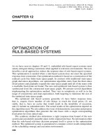
Example. Three-process mutual exclusion problem: Figure 8.1 shows the Petri
net of the solution to a three-process mutual exclusion problem. There are 10 places
in this net, three for each of the three tasks, and one “shared” among the three tasks.
P
T
mutex
P
P
tt
r1
n1

P
t
2
n2
cs2
cs2 r2
P
r3
r3
t
P
n2
t
1
n1
cs1
r1 cs1
T
tt
r2
P
P
t
cs3
P
3
T
cs3
n3
P

n3
t
Figure 8.1 Petri net of a three-process mutual exclusion algorithm.
214
TIMED PETRI NETS
A dot in place P
ni
means that task T
i
is in the non-critical region. A dot in place P
ri
means that task T
i
is in the requesting (trying) region. A dot in place P
csi
means that
task T
i
is in the critical section. There are nine transitions in this net, three for each
of the three tasks. The figure illustrates the state of the Petri net in which all three
tasks are requesting to enter the critical section. This is indicated by dots in P
r1
, P
r2
,
and P
r3
.
There are three enabled transitions in this net, t
cs1

, t
cs2
,andt
cs3
, since the input
places of each transition contain tokens. The dot in place P
mutex
indicates that one
token (privilege) is available to grant to one task to enter and execute the critical
section. The task to obtain this privilege is selected nondeterministically. Suppose
task T
1
is selected, then the transition t
cs1
fires by removing the tokens from both
of its input places and then putting a token in its output place P
cs1
, indicating that
task T
1
is executing the critical section. Note that transitions t
cs2
and t
cs3
are now
disabled since the token in P
mutex
has been removed by the firing of t
cs1
.

After task T
1
finishes executing its critical section, it goes back to its non-critical
region. This is modeled by firing transition t
n1
, which removes the token in input
place P
cs1
, and then putting a token in its output place P
n1
and a token in its output
place P
mutex
. Now either T
2
and T
3
may be selected to enter the critical section since
transitions t
cs2
and t
cs3
become enabled.
Given an initial state, the reachability set of a Petri net is the set of all states
reachable from the initial state by a sequence of transition firings. To construct the
reachability graph corresponding to a reachability set, we can represent each state by
a node and add a directed edge from state s
1
to state s
2

if firing a transition enabled
in state s
1
leads the net to state s
2
.
8.2 PETRI NETS WITH TIME EXTENSIONS
Classical Petri nets cannot express the passage of time, such as durations and time-
outs. The tokens are also anonymous and thus cannot model named items. They
also lack hierarchical decomposition or abstraction mechanisms to properly model
large systems. To model realistic real-time systems, several extended versions of
Petri nets have been proposed to deal with timing constraints. There are basically
two approaches: one associates the notions of time to transitions and the other asso-
ciates time values to places.
[Ramchandani, 1974] associated a finite firing time to each transition in a classi-
cal Petri net to yield timed Petri nets (TdPNs). More precisely, the firing of a transi-
tion now takes time and a transition must fire as soon as it is enabled. TdPNs have
been used mainly for performance evaluation. Shortly thereafter, [Merlin and Farber,
1976] developed a more general class of nets called time Petri nets (TPNs). These
are Petri nets with labels: two values of time expressed as real numbers, x and y,are
associated with each transition where x < y. x is the delay after which and y is the
deadline by which to fire the enabled transition. A TPN can model a TdPn but not
vice versa.
PETRI NETS WITH TIME EXTENSIONS
215
8.2.1 Timed Petri Nets
A TdPN is formally defined as a tuple (P, T, F, V, M
0
, D) where
P is a finite set of places;

T is a finite, ordered set of transitions t
1
,...,t
m
;
B is the backward incidence function B : T × P → N ,whereN is tghe set of
nonnegative integers;
V : F → (P, T, F) is the arc multiplicity;
D : T → N assigns to every transition t
I
a nonnegative real number N indicating
the duration of the firing of t
I
;and
M
0
is the initial marking.
A TdPN follows the following earliest firing schedule transition rule: An enabled
transition at a time k must fire at this time if there is no conflict. Transitions with
no firing durations (D(t) = 0) fire first. When a transition starts firing at time t it
removes the corresponding number of tokens from its input places at time t and adds
the corresponding number of tokens to its output places at time k + D(t).Atany
time, a maximal set of concurrently enabled transitions (maximal step) is fired.
8.2.2 Time Petri Nets
A TPN is formally defined as a tuple (P, T, B, F, M
0
, S)where
P is a finite set of places;
T is a finite, ordered set of transitions t
1

, t
2
,...,t
m
;
B is the backward incidence function B : T × P → N ,whereN is the set of
nonnegative integers;
F is the forward incidence function F : T × P → N ;
M
0
is the initial marking function M
0
: P → N ;
S is the static interval mapping
S : T → Q
∗
× (Q
∗
∪∞),whereQ
∗
is the set of positive rational numbers.
[Merlin and Farber, 1976] specifies timing constraints on a transition t
i
using
constrained static rational values as follows.
Static Firing Interval: Suppose α
i
S
and β
i

S
are rational numbers, then
S(t
i
) = (α
i
S
,β
i
S
),
where 0 ≤ α
S
< ∞, 0 ≤ β
S
≤∞,andα
S
≤ β
S
if β
S
=∞or α
S
<β
S
if β
S
=∞.
The interval (α
i

S
,β
i
S
) is the static firing interval for transition t
i
, indicated by the
superscript S,whereα
i
S
is the static earliest firing time (EFT) and β
S
is the static
216
TIMED PETRI NETS
latest firing time (LFT). In general, for states other than the initial state, the firing in-
tervals in the firing domain will be different from the static intervals. These dynamic
lower and upper bounds are denoted α
i
and β
i
, respectively, and are called simply
EFT and LFT, respectively.
Both the static and dynamic lower and upper bounds are relative to the instant at
which t
i
is enabled. If t
i
is enabled at time θ, then while t
i

is continuously enabled,
it must fire only in the time interval between θ + α
i
S
(or θ + α
i
)andθ + β
i
S
(or
θ + β
i
).
For modeling real-time systems, EFT corresponds to the delay before a transition
can be fired, and LFT is the deadline by which a transition must fire. In Merlin’s
model, time can be either discrete or dense. Also, the firing of a transition happens
instantaneously; that is, firing a transition takes no time.
If there is no time interval associated with a transition, this transition is a classical
Petri net transition and the time interval can be defined as α
i
S
= 0,β
i
S
=∞.
This indicates that an enabled transition may fire, but is not forced (required) to fire.
Therefore, TPNs are timed restrictions of Petri nets.
TPN States: A state S of a TPN is a pair (M, I ) where M is a marking, and I is a
firing interval set which is a vector of possible firing times.
For each transition enabled by marking M, a corresponding entry exists of the form

(EFT,LFT) in I . Since the number of transitions enabled by a marking varies, the
number of entries in I also varies as the Petri net runs. If the enabled transitions are
ordered (numbered) in I , then entry i in I is the i th transition in the set of transitions
enabled by M.
Example. For the example Petri net in Figure 8.1, M = P
r1
(1), P
r2
(1), P
r3
(1),
P
mutex
(1). Four places are marked, each containing one token. There are three en-
abled transitions: t
cs1
, t
cs2
,andt
cs3
. Suppose I has the following three time interval
entries: (1, 6)(2, 7)(3, 8). Transition t
cs1
may fire at any time between 1 and 6.
Transition t
cs2
may fire at any time between 2 and 7. Transition t
cs3
may fire at any
time between 3 and 8. Note that as soon as one transition fires, the other two become

disabled.
Conditions for Firing Enabled Transitions
Again, assuming the current TPN
state S = (M, I ), a subset of the set of all enabled transitions may fire owing to the
EFT and LFT timing restrictions on these transitions. Formally, a transition t
i
is
firable from state S at time θ + δ iff both of the following conditions hold:
1. t
i
is enabled by marking M at time θ under the usual enabling condition of
classical Petri nets; that is, ∀ p(M( p) ≥ B(t
i
, p));and
2. δ is at least EFT of t
i
and at most the minimum of the LFTs of all transitions
enabled by M; that is, EFT of t
i
≤ δ ≤ min(LFTs of t
k
enabled by M).
PETRI NETS WITH TIME EXTENSIONS
217
The reason for condition (2) is as follows. Suppose t
j
is the transition with the
smallest LFT among all enabled transitions. Then t
j
must fire at time δ = LFT

j
if
no other enabled transition has fired, modifying the marking and thus the state of the
TPN.
The firing of a transition t
i
at relative time δ leads the TPN to a new state S

=
(M

, I

), which can be derived as follows:
1. The new marking M

is derived with the usual Petri nets rule: ∀ pM

( p) =
M

( p) − B(t
i
, p) + F(t
i
, p).
2. To derive the new set of time intervals I

, we first remove from I the intervals
associated with the transitions that are disabled after firing t

i
. Note that t
i
is
also diabled after its firing. Then we shift the remaining time intervals by δ
towards the origin of times, truncating them if necessary to obtain nonnegative
values. This corresponds to incrementing time by δ. Finally, we add to I the
static intervals of the newly enabled transitions, yielding I

. Thus the domain
of the new state is the product of the time intervals of the remaining enabled
transitions and those of the newly enabled transitions.
We use the following notation to denote that transition t
i
is firable from state S at
time δ and its firing leads to state S

:
S
(t
i
,δ)
−→ S

.
Firing Schedule: A firing schedule is a sequence of pairs (t
i
,δ
1
)(t

2
,δ
2
) ···
(t
n
,δ
n
). This schedule is feasible from state S iff states exist such that
S
(t
1
,δ
1
)
−→ S
1
(t
2
,δ
2
)
−→ S
2
··· −→ S
n−1
(t
n
,δ
n

)
−→ S
n
.
With this definition, we can construct the reachability graph to characterize the be-
havior of a TPN. However, as in other state space graphs, this reachability graph may
have an infinite number of states and hence cannot be constructed in practice. Some
simulation techniques that do not require the construction of the entire reachability
graph have been proposed but are not appropriate for the analysis of safety-critical
real-time systems. Later in this chapter we describe an efficient exhaustive analysis
technique for a class of TPNs.
Example. For the example Petri net in Figure 8.1,
M
0
= P
r1
(1), P
r2
(1), P
r3
(1), P
mutex
(1).
I
0
= (1, 8)(2, 7)(3, 6).
Therefore, any one of the three transitions t
cs1
, t
cs2

, t
cs3
may fire according to the
following timing restrictions. Transition t
cs1
may fire in the period between relative
time 1 (the EFT of (1,8)) and relative time 6 (the minimum of the LFTs (6,7,8) of the
218
TIMED PETRI NETS
intervals for the three enabled transitions). Similarly, transition t
cs2
may fire in the
period between relative time 2 (the EFT of (2, 7)) and relative time 6; and transition
t
cs3
may fire in the period between relative time 3 (the EFT of (3, 6)) and relative
time 6. The choice of which transition to fire is nondeterministic.
Thus at any time δ
1
within the infinite number of real values in interval (1, 6),
firing t
cs1
leads to state S
1
= (M
1
, I
1
):
M

1
= p
cs1
(1), p
r2
(1), p
r3
(1) and
I
1
= (1, 2).
Notice transitions t
cs2
and t
cs3
have been disabled by the firing of t
cs1
and thus
their associated time intervals are removed from I . Also, transition t
cs1
is disabled
after its own firing. Transition t
n1
has enabled t
cs1
and so the associated time interval
(1, 2) is added to I .
Next, there is only one enabled transition to fire. Firing t
n1
leads to state S

2
=
(M
2
, I
2
):
M
1
= p
n1
(1), p
r2
(1), p
r3
(1) and
I
1
= (2, 4).
8.2.3 High-Level Timed Petri Nets
High-level timed Petri nets (HLTPNs), or time environment/relationship nets
(TERNs) [Ghezzi et al., 1991], integrate functional and temporal descriptions in
the same model. In particular, HLTPNs provide features that can precisely model
the identities of a system’s components as well as their logical and timing properties
and relationships. A HLTPN is a classical Petri net augmented with the following
features.
For each place, a restriction exists on the type of tokens that can mark it; for
example, each place has one or more types. If any type of token can mark a place,
then this place has the same meaning as in a classical Petri net. Each token has a
time-stamp indicating its creation time (or birth date) and a data structure for storing

its associated data.
Each transition has a predicate that determines when and how the transition is
enabled. This is similar to a transition in TPNs but is more elaborate. In HLTPNs, this
predicate expresses constraints based on the values of the data structures and time-
stamps of the tokens in the input places. A transition also has an action that specifies
the values of the data to be associated with the tokens produced by the transition
firing. This action depends on the data and time-stamps of the tokens removed by
the firing. Finally, a transition has a time function that specifies the minimum and
maximum firing times. This function depends also on the data and time-stamps of
the tokens removed by the firing. Graphically, a transition is represented by a box or
rectangle.
PETRI NETS WITH TIME EXTENSIONS
219
Environment/Relationship Nets
We first more formally describe environ-
ment/relationship (ER) nets without timing extensions. Tokens in ER nets are
environments, functions that associate values to variables. Each transition has an
associated action that specifies the types of tokens for enabling the transitions and
the types of tokens produced by the firing. More precisely, in an ER net:
1. Tokens are environments or possibly partial functions on IDand V : ID → V ,
where I is a set of identifiers and V is a set of values. ENV = V
ID
is the set
of all environments.
2. Each transition t has an associated action, which is a relationship: α(t) ⊆
ENV
k(t)
× ENV
h(t)
,wherek(t ) and h(t) are the cardinalities of the preset and

postset of transition t , respectively. The weight of each arc is 1. Also, h(t)>0
for all t. The predicate of transition t, denoted π(t), is the projection of α(t)
on ENV
k(t)
.
3. A marking M is an assignment of multisets of environments to places.
4. In a marking M, a transition t is enabled iff for every input place p
i
of t, at least
one token env
i
exists such that the enabling tuple env
1
,...,env
k(t)
∈π(t).
More than one enabling tuple may exist for transition t, and a token may appear
in more than one enabling tuple.
5. A firing is a triple x =enab, t, prod, where enab is the input tuple, prod is
the output tuple, and enab, prod∈α(t ).
6. In a marking M, the firing enab, t, prod occurs by removing the enabling
tuple enab from the input places of transition T and storing the tuple prod in
the output places of transition T , thus producing a new marking, M

.
7. A firing sequence starting from marking M
0
is a finite sequence of firings,
enab
1

, t
1
, prod
1
, ···, enab
n
, t
n
, prod
n
,
where t
1
is enabled in M
0
by enab
1
; each t
i
, i = 2,...,n, is enabled in M
i−1
by the firing enab
i−1
, t
i−1
, prod
i−1
 and its firing produces M
i
.

Example. Figure 8.2 shows a sample ER net, which consists of three places and one
transition with an action:
token
1
={x, −1, y, 2}
token
2
={x, 2, y, 2}
token
3
={x, 1, y, 2}
act ={p
1
, p
2
, p
3
| p
1
.x < p
2
.x ∧ p
1
.y = p
2
.y ∧
p
3
.x = p
1

.x + p
2
.x ∧ p
3
.y = p
1
.y}
Only tokens token
1
and token
3
satisfy the predicate in the action act associated with
the transition t since −1 < 1and2 = 2. Hence only these two tokens form an
220
TIMED PETRI NETS
PP
P
1
2
1
2
3
act
t
3
token = {<x, −1>, <y, 2>}
token = {<x, 1>, <y, 2>}
token
token
token

1
3
2
token = {<x, 2>, <y, 2>}
Figure 8.2 Sample ER net.
enabling tuple for transition t. Firing t produces an environment in place p
3
where
p
3
.x =−1 + 1 = 0and p
3
.y = 2.
In the next section, we describe in detail time ER nets, the most recent of the three
time-extended Petri nets introduced here.
8.3 TIME ER NETS
To extend ER nets to specify the notions of time, a variable chronos is introduced
[Ghezzi et al., 1991] to represent the time-stamp of the token in each environment.
This time-stamp gives the time when the token is produced. The time-stamps of the
tokens put in output places are produced by the actions associated with the transitions
and are based on the selected input enabling a tuple’s environments’ values.
The variable chronos can take on nonnegative real numbers when used in a con-
tinuous time model, or nonnegative integers when used in a discrete time model.
This concept of a time-stamp assigned to a token when it is produced is similar to
the time value given by the occurrence function in real-time logic and the time value
τ indicating the time of the corresponding event occurrence in timed languages and
automata. An occurrence function assigns a time to the occurrence of an instance of
an event. τ denotes the occurrence time of an event ρ in the pair (ρ, τ ).
To enforce time restrictions on chronos, we need the following axioms.
Local Monotonicity Axiom: Let c

1
be the value of chronos in the environments
removed by (before) any firing, and let c
2
be the value of chronos in the environments
produced by (after) this firing. Then, c
1
≤ c
2
.
Constraint on Time-Stamps Axiom: The values of all elements of the tuple prod
in any firing x =enab, t, prod are equal to chronos. This time of the firing is
denoted as time(x).
TIME ER NETS
221
Firing Sequence Monotonicity Axiom: The times of the firings are monotonically
nondecreasing with respect to their occurrence in any firing sequence.
Equivalent Firing Sequences: Given an initial marking M
0
, two firing sequences s
and s

are equivalent iff s is a permutation of s

.
Time-Ordered Firing Sequence: A firing sequence t
1
,...,t
n
 is time-ordered in

an ER net satisfying the constraint on time-stamps axiom iff for every i, j, i < j →
time(t
i
) ≤ time(t
j
).
For each firing sequence s with an initial marking M
0
in an ER net satisfying the
local monotonicity axiom and the constraint on time-stamps axiom, a time-ordered
firing sequence s

exists equivalent to s.
Time ER Net (TERN): An ER net satisfying both the local monotonicity axiom
and the constraint on time-stamps axiom, and with a variable chronos in every envi-
ronment, is a TERN.
Example. Figure 8.3 shows a partial TERN for a smart traffic light system at an in-
tersection. The traffic light for cars turns green when a car arrives at the intersection.
P
P
2
3
P
1
no pedestrian
for cars
car(s) at
intersection
light turns green
PP

car stalls
t
car crosses
intersection
t
t
5
4
1
2
3
Figure 8.3 Partial TERN for a smart traffic light system.