Pricing Exotic Options

Chapter 20
Pricing Exotic Options
20.1 Reflection principle for Brownian motion
Without drift.
Define
M T  = max
0tT
B t:
Then we have:
IP fM T  m;BTbg
=IPfBT2m,bg
=
1
p
2T
Z
1
2m,b
exp

,
x
2
2T

dx; m0;bm
So the joint density is
IP fM T  2 dm; B T  2 dbg = ,
@
2
@m @b


1
p
2T
Z
1
2m,b
exp

,
x
2
2T

dx
!
dm db
= ,
@
@m

1
p
2T
exp

,
2m , b
2
2T

!
dm db;
=
22m , b
T
p
2T
exp

,
2m , b
2
2T

dm db; m0;b  m:
With drift. Let
e
B t=t + Bt;
209
210
shadow path
m
Brownian motion
2m-b
b
Figure 20.1: Reflection Principle for Brownian motion without drift
m=b
b
m
(B(T), M(T)) lies in here

Figure 20.2: Possible values of
B T ;MT
.
CHAPTER 20. Pricing Exotic Options
211
where
B t; 0  t  T
, is a Brownian motion (without drift) on
; F ; P
.Define
Z T  = expf,B T  ,
1
2

2
T g
= expf, B T +T +
1
2

2
Tg
= expf,
e
B t+
1
2

2
Tg;

f
IPA=
Z
A
ZTdIP; 8A 2F:
Set
f
M T  = max
0tT
e
B T :
Under
f
IP;
e
B
is a Brownian motion (without drift), so
f
IP f
f
M T  2 d ~m;
e
B T  2 d
~
bg =
22 ~m ,
~
b
T
p

2T
exp

,
2 ~m ,
~
b
2
2T

d ~md
~
b; ~m0;
~
b ~m:
Let
h~m;
~
b
be a function of two variables. Then
IEh
f
M T ;
e
BT  =
f
IE
h
f
M T ;

e
B T 
Z T 
=
f
IE
h
h
f
M T ;
e
B T  expf
e
B T  ,
1
2

2
T g
i
=
~m=1
Z
~m=0
~
b=~m
Z
~
b=,1
h~m;

~
b expf
~
b ,
1
2

2
T g
f
IP f
f
M T  2 d ~m;
e
B T  2 d
~
bg:
But also,
IEh
f
M T ;
e
BT  =
~m=1
Z
~m=0
~
b=~m
Z
~

b=,1
h~m;
~
b IPf
f
MT 2 d~m;
e
BT 2 d
~
bg:
Since
h
is arbitrary, we conclude that
(MPR)
IP f
f
M T  2 d ~m;
e
B T  2 d
~
bg
= expf
~
b ,
1
2

2
T g
f

IP f
f
M T  2 d ~m;
e
B T  2 d
~
bg
=
22 ~m ,
~
b
T
p
2T
exp

,
2 ~m ,
~
b
2
2T

: expf
~
b ,
1
2

2

T gd ~md
~
b; ~m0;
~
b ~m:
212
20.2 Up and out European call.
Let
0 K L
be given. The payoff at time
T
is
S T  , K 
+
1
fS

T Lg
;
where
S

T  = max
0tT
S t:
To simplify notation, assume that
IP
is already the risk-neutral measure, so the value at time zero of
the option is
v 0;S0 = e

,rT
IE
h
ST  , K 
+
1
fS

T Lg
i
:
Because
IP
is the risk-neutral measure,
dS t=rS t dt + S t dB t
S t=S
0
expfBt+r,
1
2

2
tg
= S
0
exp
8








:

2
6
6
6
4
B t+

r

,

2

| z 

t
3
7
7
7
5
9




=



;
= S
0
expf
e
B tg;
where
 =

r

,

2

;
e
B t=t + Bt:
Consequently,
S

t=S
0
expf
f

M tg;
where,
f
M t = max
0ut
e
B u:
We compute,
v 0;S0 = e
,rT
IE
h
ST  , K 
+
1
fS

T Lg
i
= e
,rT
IE


S 0 expf
e
B T g, K

+
1

fS0 expf
e
M T g Lg

= e
,rT
IE
"

S 0 expf
e
B T g,K

1

e
BT
1

log
K
S 0
| z 
~
b
;
e
M T 
1


log
L
S 0
| z 
~m


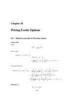
CHAPTER 20. Pricing Exotic Options
213
(B(T), M(T)) lies in here
M(T)
B(T)
x
y
b
m
~
~
~
~
x=y
Figure 20.3: Possible values of
e
B T ;
f
M T 
.
We consider only the case
S 0  KL;
so

0 
~
b ~m:
The other case,
KS0  L
leads to
~
b0  ~m
and the analysis is similar.
We compute
R
~m
~
b
R
~m
x
: : : dy dx
:
v 0;S0 = e
,rT
Z
~m
~
b
Z
~m
x
S0 expfxg, K
22y , x

T
p
2T
exp

,
2y , x
2
2T
+ x ,
1
2

2
T

dy dx
= ,e
,rT
Z
~m
~
b
S0 expfxg,K
1
p
2T
exp

,

2y , x
2
2T
+ x ,
1
2

2
T





y=~m
y=x
dx
= e
,rT
Z
~m
~
b
S 0 expfxg,K
1
p
2T
"
exp


,
x
2
2T
+ x ,
1
2

2
T

, exp

,
2 ~m , x
2
2T
+ x ,
1
2

2
T

dx
=
1
p
2T
e

,rT
S 0
Z
~m
~
b
exp

x ,
x
2
2T
+ x ,
1
2

2
T

dx
,
1
p
2T
e
,rT
K
Z
~m
~

b
exp

,
x
2
2T
+ x ,
1
2

2
T

dx
,
1
p
2T
e
,rT
S 0
Z
~m
~
b
exp

x ,
2 ~m , x

2
2T
+ x ,
1
2

2
T

dx
+
1
p
2T
e
,rT
K
Z
~m
~
b
exp

,
2 ~m , x
2
2T
+ x ,
1
2


2
T

dx:
The standard method for all these integrals is to complete the square in the exponent and then
recognize a cumulative normal distribution. We carry out the details for the first integral and just