Pricing in terms ofMarket Probabilities_ The Radon-Nikodym Theorem
Bạn đang xem bản rút gọn của tài liệu. Xem và tải ngay bản đầy đủ của tài liệu tại đây (183.42 KB, 8 trang )
Chapter 9
Pricing in terms of Market Probabilities:
The Radon-Nikodym Theorem.
9.1 Radon-Nikodym Theorem
Theorem 1.27 (Radon-Nikodym) Let IP and
f
IP
be two probability measures on a space
; F
.
Assume that for every
A 2F
satisfying
IP A=0
, we also have
f
IP A=0
. Then we say that
f
IP
is absolutely continuous with respect to IP. Under this assumption, there is a nonegative random
variable
Z
such that
f
IP A=
Z
A
ZdIP; 8A 2F;
(1.1)
and
Z
is called the Radon-Nikodym derivative of
f
IP
with respect to IP.
Remark 9.1 Equation (1.1) implies the apparently stronger condition
f
IEX = IEXZ
for every random variable
X
for which
IE jXZj 1
.
Remark 9.2 If
f
IP
is absolutely continuous with respect to IP, and IP is absolutely continuous with
respect to
f
IP
, we say that IPand
f
IP
are equivalent. IPand
f
IP
are equivalent if and only if
IP A=0
exactly when
f
IP A=0; 8A2F:
If IPand
f
IP
are equivalent and
Z
is the Radon-Nikodym derivative of
f
IP
w.r.t. IP, then
1
Z
is the
Radon-Nikodym derivative of IP w.r.t.
f
IP
, i.e.,
f
IEX = IEXZ 8X;
(1.2)
IEY =
f
IEY:
1
Z
8Y:
(1.3)
(Let
X
and
Y
be related by the equation
Y = XZ
to see that (1.2) and (1.3) are the same.)
111
112
Example 9.1 (Radon-Nikodym Theorem) Let
=fHH; HT; T H; T T g
, the set of coin toss sequences
of length 2. Let
P
correspond to probability
1
3
for
H
and
2
3
for
T
,andlet
e
IP
correspond to probability
1
2
for
H
and
1
2
for
T
.Then
Z ! =
e
IP!
IP!
,so
Z HH=
9
4
;ZHT =
9
8
;ZTH=
9
8
;ZTT=
9
16
:
9.2 Radon-Nikodym Martingales
Let
be the set of all sequences of
n
coin tosses. Let IP be the market probability measure and let
f
IP
be the risk-neutral probability measure. Assume
IP ! 0;
f
IP ! 0; 8! 2 ;
so that IPand
f
IP
are equivalent. The Radon-Nikodym derivative of
f
IP
with respect to IPis
Z ! =
f
IP!
IP!
:
Define the IP-martingale
Z
k
4
= IE Z jF
k
;k=0;1;::: ;n:
We can check that
Z
k
is indeed a martingale:
IE Z
k+1
jF
k
= IE IE Z jF
k+1
jF
k
= IE Z jF
k
= Z
k
:
Lemma 2.28 If
X
is
F
k
-measurable, then
f
IEX = IEXZ
k
.
Proof:
f
IEX = IEXZ
= IE IEXZjF
k
= IE X:IE ZjF
k
= IE XZ
k
:
Note that Lemma 2.28 implies that if
X
is
F
k
-measurable, then for any
A 2F
k
,
f
IEI
A
X=IEZ
k
I
A
X;
or equivalently,
Z
A
Xd
f
IP =
Z
A
XZ
k
dIP:
CHAPTER 9. Pricing in terms of Market Probabilities
113
0
1
1
2
2
2
2
Z = 1
Z (H) = 3/2
Z (T) = 3/4
Z (HH) = 9/4
Z (HT) = 9/8
Z (TH) = 9/8
Z (TT) = 9/16
2/3
1/3
1/3
2/3
1/3
2/3
Figure 9.1: Showing the
Z
k
values in the2-periodbinomialmodel example. The probabilitiesshown
are for IP, not
f
IP
.
Lemma 2.29 If
X
is
F
k
-measurable and
0 j k
,then
f
IE X jF
j
=
1
Z
j
IEXZ
k
jF
j
:
Proof: Note first that
1
Z
j
IE XZ
k
jF
j
is
F
j
-measurable. So for any
A 2F
j
,wehave
Z
A
1
Z
j
IE XZ
k
jF
j
d
f
IP =
Z
A
IE XZ
k
jF
j
dIP
(Lemma 2.28)
=
Z
A
XZ
k
dIP
(Partial averaging)
=
Z
A
Xd
f
IP
(Lemma 2.28)
Example 9.2 (Radon-Nikodym Theorem, continued) We show in Fig. 9.1 the values of the martingale
Z
k
.
We always have
Z
0
=1
,since
Z
0
= IEZ =
Z
ZdIP =
e
IP =1:
9.3 The State Price Density Process
In order to express the value of a derivative security in terms of the market probabilities, it will be
useful to introduce the following state price density process:
k
=1+r
,k
Z
k
;k=0;::: ;n:
114
We then have the following pricing formulas: For a Simple European derivative security with
payoff
C
k
at time
k
,
V
0
=
f
IE
h
1 + r
,k
C
k
i
= IE
h
1 + r
,k
Z
k
C
k
i
(Lemma 2.28)
= IE
k
C
k
:
More generally for
0 j k
,
V
j
= 1 + r
j
f
IE
h
1 + r
,k
C
k
jF
j
i
=
1 + r
j
Z
j
IE
h
1 + r
,k
Z
k
C
k
jF
j
i
(Lemma 2.29)
=
1
j
IE
k
C
k
jF
j
Remark 9.3
f
j
V
j
g
k
j =0
is a martingale under IP, as we can check below:
IE
j +1
V
j +1
jF
j
= IE IE
k
C
k
jF
j +1
jF
j
= IE
k
C
k
jF
j
=
j
V
j
:
Now for an American derivative security
fG
k
g
n
k=0
:
V
0
= sup
2T
0
f
IE 1 + r
,
G
= sup
2T
0
IE 1 + r
,
Z
G
= sup
2T
0
IE
G
:
More generally for
0 j n
,
V
j
= 1 + r
j
sup
2T
j
f
IE 1 + r
,
G
jF
j
= 1 + r
j
sup
2T
j
1
Z
j
IE 1 + r
,
Z
G
jF
j
=
1
j
sup
2T
j
IE
G
jF
j
:
Remark 9.4 Note that
(a)
f
j
V
j
g
n
j =0
is a supermartingale under IP,
(b)
j
V
j
j
G
j
8j;
CHAPTER 9. Pricing in terms of Market Probabilities
115
S = 4
0
S (H) = 8
S (T) = 2
S (HH) = 16
S (TT) = 1
S (HT) = 4
S (TH) = 4
1
1
2
2
2
2
ζ = 1.00
ζ (Η) = 1.20
ζ (Τ) = 0.6
ζ (ΗΗ) = 1.44
ζ (ΗΤ) = 0.72
ζ (ΤΗ) = 0.72
ζ (ΤΤ) = 0.36
0
1
1
2
2
2
2
1/3
2/3
1/3
2/3
1/3
2/3
Figure 9.2: Showing the state price values
k
. The probabilities shown are for IP, not
f
IP
.
(c)
f
j
V
j
g
n
j =0
is the smallest process having properties (a) and (b).
We interpret
k
by observing that
k
! IP !
is the value at time zero of a contract which pays $1
at time
k
if
!
occurs.
Example 9.3 (Radon-NikodymTheorem, continued) We illustrate the use of the valuation formulas for
European and American derivative securities in terms of market probabilities. Recall that
p =
1
3
,
q =
2
3
.The
state price values
k
are shown in Fig. 9.2.
For a European Call with strike price 5, expiration time 2, we have
V
2
HH=11;
2
HHV
2
HH=1:44 11 = 15:84:
V
2
HT =V
2
TH=V
2
TT=0:
V
0
=
1
3
1
3
15:84 = 1:76:
2
HH
1
HH
V
2
HH=
1:44
1:20
11 = 1:20 11 = 13:20
V
1
H =
1
3
13:20 = 4:40
Compare with the risk-neutral pricing formulas:
V
1
H =
2
5
V
1
HH+
2
5
V
1
HT =
2
5
11 = 4:40;
V
1
T =
2
5
V
1
TH+
2
5
V
1
TT=0;
V
0
=
2
5
V
1
H+
2
5
V
1
T=
2
5
4:40 = 1:76:
Now consider an American put with strike price 5 and expiration time 2. Fig. 9.3 shows the values of
k
5 , S
k
+
. We compute the value of the put under various stopping times
:
(0) Stop immediately: value is 1.
(1) If
HH=HT =2;TH=TT=1
,thevalueis
1
3
2
3
0:72 +
2
3
1:80 = 1:36: