Semi-Continuous Models

Chapter 12
Semi-Continuous Models
12.1 Discrete-time Brownian Motion
Let
fY
j
g
n
j =1
be a collection of independent,standard normal random variables defined on
; F ; P
,
where IPisthemarket measure. As before we denote the column vector
Y
1
;::: ;Y
n

T
by
Y
.We
therefore have for any real colum vector
u =u
1
;::: ;u
n

T
,
IEe

u
T
Y
= IE exp
8

:
n
X
j =1
u
j
Y
j
9
=
;
= exp
8

:
n
X
j =1
1
2
u
2
j
9

=
;
:
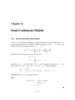
Define the discrete-time Brownian motion (See Fig. 12.1):
B
0
= 0;
B
k
=
k
X
j =1
Y
j
;k=1;::: ;n:
If we know
Y
1
;Y
2
;::: ;Y
k
, then we know
B
1
;B
2
;::: ;B
k

. Conversely, if we know
B
1
;B
2
;::: ;B
k
,
then we know
Y
1
= B
1
;Y
2
= B
2
, B
1
;::: ;Y
k
= B
k
, B
k,1
. Define the filtration
F
0
= f; g;
F

k
=  Y
1
;Y
2
;::: ;Y
k
=B
1
;B
2
;::: ;B
k
;k=1;::: ;n:
Theorem 1.34
fB
k
g
n
k=0
is a martingale (under IP).
Proof:
IE B
k+1
jF
k
 = IE Y
k+1
+ B
k

jF
k

= IEY
k+1
+ B
k
= B
k
:
131
132
Y
Y
Y
Y
1
2
3
4
k
B
k
0
12 34
Figure 12.1: Discrete-time Brownian motion.
Theorem 1.35
fB
k
g

n
k=0
is a Markov process.
Proof: Note that
IE hB
k+1
jF
k
=IEhY
k+1
+ B
k
jF
k
:
Use the Independence Lemma. Define
g b= IEhY
k+1
+ b=
1
p
2
Z
1
,1
hy + be
,
1
2
y

2
dy :
Then
IE hY
k+1
+ B
k
jF
k
=gB
k
;
which is a function of
B
k
alone.
12.2 The Stock Price Process
Given parameters:
  2 IR
,themean rate of return.
 0
,thevolatility.
 S
0
 0
, the initial stock price.
The stock price process is then given by
S
k
= S

0
exp
n
B
k
+,
1
2

2
k
o
;k=0;::: ;n:
Note that
S
k+1
= S
k
exp
n
Y
k+1
+,
1
2

2

o
;

CHAPTER 12. Semi-Continuous Models
133
IE S
k+1
jF
k
 = S
k
IE e
Y
k+1
jF
k
:e
,
1
2

2
= S
k
e
1
2

2
e
,
1
2


2
= e

S
k
:
Thus
 = log
IE S
k+1
jF
k

S
k
= log IE

S
k+1
S
k




F
k

;

and
var

log
S
k+1
S
k

=var

Y
k+1
+,
1
2

2


= 
2
:
12.3 Remainder of the Market
The other processes in the market are defined as follows.
Money market process:
M
k
= e
rk

;k=0;1;::: ;n:
Portfolio process:
 
0
; 
1
;::: ;
n,1
;

Each

k
is
F
k
-measurable.
Wealth process:
 X
0
given, nonrandom.

X
k+1
= 
k
S
k+1
+ e
r

X
k
, 
k
S
k

= 
k
S
k+1
, e
r
S
k
+e
r
X
k

Each
X
k
is
F
k
-measurable.
Discounted wealth process:
X
k+1

M
k+1
=
k

S
k+1
M
k+1
,
S
k
M
k

+
X
k
M
k
:
12.4 Risk-Neutral Measure
Definition 12.1 Let
f
IP
be a probability measure on
; F 
, equivalent to the market measure IP. If
n
S

k
M
k
o
n
k =0
is a martingale under
f
IP
, we say that
f
IP
is a risk-neutral measure.
134
Theorem 4.36 If
f
IP
is a risk-neutral measure, then every discounted wealth process
n
X
k
M
k
o
n
k=0
is
a martingale under
f
IP

, regardless of the portfolio process used to generate it.
Proof:
f
IE

X
k+1
M
k+1




F
k

=
f
IE


k

S
k+1
M
k+1
,
S
k

M
k

+
X
k
M
k




F
k

= 
k

f
IE

S
k+1
M
k+1




F

k

,
S
k
M
k

+
X
k
M
k
=
X
k
M
k
:
12.5 Risk-Neutral Pricing
Let
V
n
be the payoff at time
n
,andsayitis
F
n
-measurable. Note that
V

n
may be path-dependent.
Hedging a short position:

Sell the simple European derivative security
V
n
.

Receive
X
0
at time 0.

Construct a portfolio process

0
;::: ;
n,1
which starts with
X
0
and ends with
X
n
= V
n
.

If there is a risk-neutral measure

f
IP
,then
X
0
=
f
IE
X
n
M
n
=
f
IE
V
n
M
n
:
Remark 12.1 Hedging in this “semi-continuous” model is usually not possible because there are
not enough trading dates. This difficulty will disappear when we go to the fully continuous model.
12.6 Arbitrage
Definition 12.2 An arbitrage is a portfolio which starts with
X
0
=0
and ends with
X
n

satisfying
IP X
n
 0 = 1;IPX
n
0  0:
(IP here is the market measure).
Theorem 6.37 (Fundamental Theorem of Asset Pricing: Easy part) Ifthere is a risk-neutralmea-
sure, then there is no arbitrage.
CHAPTER 12. Semi-Continuous Models
135
Proof: Let
f
IP
be a risk-neutral measure, let
X
0
=0
,andlet
X
n
be the final wealth corresponding
to any portfolio process. Since
n
X
k
M
k
o
n

k=0
is a martingale under
f
IP
,
f
IE
X
n
M
n
=
f
IE
X
0
M
0
=0:
(6.1)
Suppose
IP X
n
 0 = 1
.Wehave
IP X
n
 0 = 1 = IP X
n
 0 = 0 =

f
IP X
n
 0 = 0 =
f
IP X
n
 0 = 1:
(6.2)
(6.1) and (6.2) imply
f
IP X
n
=0=1
.Wehave
f
IP X
n
=0=1=
f
IPX
n
0=0=IPX
n
0=0:
This is not an arbitrage.
12.7 Stalking the Risk-Neutral Measure
Recall that
 Y
1

;Y
2
;::: ;Y
n
are independent, standard normal random variables on some probabilityspace
; F ; P
.
 S
k
= S
0
exp
n
B
k
+,
1
2

2
k
o
.

S
k+1
= S
0
exp
n

 B
k
+ Y
k+1
+ ,
1
2

2
k +1
o
= S
k
exp
n
Y
k+1
+,
1
2

2

o
:
Therefore,
S
k+1
M
k+1

=
S
k
M
k
: exp
n
Y
k+1
+,r ,
1
2

2

o
;
IE

S
k+1
M
k+1




F
k


=
S
k
M
k
:IE exp fY
k+1
gjF
k
:expf , r ,
1
2

2
g
=
S
k
M
k
: expf
1
2

2
g: expf , r ,
1
2

2

g
= e
,r
:
S
k
M
k
:
If
 = r
, the market measure is risk neutral. If
 6= r
, we must seek further.