Modeling, Measurement and Control P18
Bạn đang xem bản rút gọn của tài liệu. Xem và tải ngay bản đầy đủ của tài liệu tại đây (1.96 MB, 62 trang )
18
The Dynamics of the
Class 1 Shell
Tensegrity Structure
18.1 Introduction
18.2 Tensegrity Definitions
A Typical Element • Rules of Closure for the Shell Class
18.3 Dynamics of a Two-Rod Element
18.4 Choice of Independent Variables and
Coordinate Transformations
18.5 Tendon Forces
18.6 Conclusion
Appendix 18.A Proof of Theorem 18.1
Appendix 18.B Algebraic Inversion of the Q Matrix
Appendix 18.C General Case for (n, m) = (i, 1)
Appendix 18.D Example Case (n,m) = (3,1)
Appendix 18.E Nodal Forces
Abstract
A tensegrity structure is a special truss structure in a stable equilibrium with selected members
designated for only tension loading, and the members in tension forming a continuous network of
cables separated by a set of compressive members. This chapter develops an explicit analytical
model of the nonlinear dynamics of a large class of tensegrity structures constructed of rigid rods
connected by a continuous network of elastic cables. The kinematics are described by positions
and velocities of the ends of the rigid rods; hence, the use of angular velocities of each rod is avoided.
The model yields an analytical expression for accelerations of all rods, making the model efficient
for simulation, because the update and inversion of a nonlinear mass matrix are not required. The
model is intended for shape control and design of deployable structures. Indeed, the explicit
analytical expressions are provided herein for the study of stable equilibria and controllability, but
control issues are not treated.
18.1 Introduction
The history of structural design can be divided into four eras classified by design objectives. In the
prehistoric era, which produced such structures as Stonehenge, the objective was simply to oppose
gravity, to take static loads. The classical era, considered the dynamic
response and placed design
constraints on the eigenvectors as well as eigenvalues. In the modern era, design constraints could
be so demanding that the dynamic response objectives require feedback control. In this era, the
Robert E. Skelton
University of California, San Diego
Jean-Paul Pinaud
University of California, San Diego
D. L. Mingori
University of California, Los Angeles
8596Ch18Frame Page 389 Wednesday, November 7, 2001 12:18 AM
© 2002 by CRC Press LLC
control discipline followed the classical structure design, where the structure and control disciplines
were ingredients in a multidisciplinary system design, but no interdisciplinary tools were developed
to integrate the design of the structure and the control. Hence, in this modern era, the dynamics of
the structure and control were not cooperating to the fullest extent possible. The post-modern era
of structural systems is identified by attempts to unify the structure and control design for a common
objective.
The ultimate performance capability of many new products and systems cannot be achieved until
mathematical tools exist that can extract the full measure of cooperation possible between the
dynamics of all components (structural components, controls, sensors, actuators, etc.). This requires
new research. Control theory describes how the design of one component (the controller) should
be influenced by the (given) dynamics of all other components. However, in systems design, where
more than one component remains to be designed, there is inadequate theory to suggest how the
dynamics of two or more components should influence each other at the design stage. In the future,
controlled structures will not be conceived merely as multidisciplinary design steps, where a plate,
beam, or shell is first designed, followed by the addition of control actuation. Rather, controlled
structures will be conceived as an interdisciplinary process in which both material architecture and
feedback information architecture will be jointly determined. New paradigms for material and
structure design might be found to help unify the disciplines. Such a search motivates this work.
Preliminary work on the integration of structure and control design appears in Skelton
1,2
and
Grigoriadis et al.
3
Bendsoe and others
4-7
optimize structures by beginning with a solid brick and deleting finite
elements until minimal mass or other objective functions are extremized. But, a very important
factor in determining performance is the paradigm used for structure design. This chapter describes
the dynamics of a structural system composed of axially loaded compression members and tendon
members that easily allow the unification of structure and control functions. Sensing and actuating
functions can sense or control the tension or the length of tension members. Under the assumption
that the axial loads are much smaller than the buckling loads, we treat the rods as rigid bodies.
Because all members experience only axial loads, the mathematical model is more accurate than
models of systems with members in bending. This unidirectional loading of members is a distinct
advantage of our paradigm, since it eliminates many nonlinearities that plague other controlled
structural concepts: hysteresis, friction, deadzones, and backlash.
It has been known since the middle of the 20th century that continua cannot explain the strength
of materials. While science can now observe at the nanoscale to witness the architecture of materials
preferred by nature, we cannot yet design or manufacture manmade materials that duplicate the
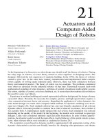
incredible structural efficiencies of natural systems. Nature’s strongest fiber, the spider fiber,
arranges simple nontoxic materials (amino acids) into a microstructure that contains a continuous
network of members in tension (amorphous strains) and a discontinuous set of members in com-
pression (the
β
-pleated sheets in Figure 18.1).
8,9
This class of structure, with a continuous network of tension members and a discontinuous
network of compression members, will be called a Class 1 tensegrity structure. The important
lessons learned from the tensegrity structure of the spider fiber are that
1. Structural members never reverse their role. The compressive members never take tension
and, of course, tension members never take compression.
2. Compressive members do not touch (there are no joints in the structure).
3. Tensile strength is largely determined by the local topology of tension and compressive
members.
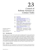
Another example from nature, with important lessons for our new paradigms is the carbon
nanotube often called the Fullerene (or Buckytube), which is a derivative of the Buckyball. Imagine
8596Ch18Frame Page 390 Wednesday, November 7, 2001 12:18 AM
© 2002 by CRC Press LLC
a 1-atom thick sheet of a graphene, which has hexagonal holes due to the arrangements of material
at the atomic level (see Figure 18.2). Now imagine that the flat sheet is closed into a tube by
choosing an axis about which the sheet is closed to form a tube. A specific set of rules must define
this closure which takes the sheet to a tube, and the electrical and mechanical properties of the
resulting tube depend on the rules of closure (axis of wrap, relative to the local hexagonal topol-
ogy).
10
Smalley won the Nobel Prize in 1996 for these insights into the Fullerenes. The spider fiber
and the Fullerene provide the motivation to construct manmade materials whose overall mechanical,
thermal, and electrical properties can be predetermined by choosing the local topology and the
rules of closure which generate the three-dimensional structure from a given local topology. By
combining these motivations from Fullerenes with the tensegrity architecture of the spider fiber,
this chapter derives the static and dynamic models of a shell class of tensegrity structures. Future
papers will exploit the control advantages of such structures. The existing literature on tensegrity
deals mainly
11-23
with some elementary work on dynamics in Skelton and Sultan,
24
Skelton and
He,
25
and Murakami et al.
26
FIGURE 18.1
Nature’s strongest fiber: the Spider Fiber. (From Termonia, Y.,
Macromolecules
, 27, 7378–7381,
1994. Reprinted with permission from the American Chemical Society.)
FIGURE 18.2
Buckytubes.
amorphous
chain
β-pleated sheet
entanglement
hydrogen bond
y
z
x
6nm
8596Ch18Frame Page 391 Wednesday, November 7, 2001 12:18 AM
© 2002 by CRC Press LLC
18.2 Tensegrity Definitions
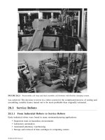
Kenneth Snelson built the first tensegrity structure in 1948 (Figure 18.3) and Buckminster Fuller
coined the word “tensegrity.” For 50 years tensegrity has existed as an art form with some archi-
tectural appeal, but engineering use has been hampered by the lack of models for the dynamics.
In fact, engineering use of tensegrity was doubted by the inventor himself. Kenneth Snelson in a
letter to R. Motro said, “As I see it, this type of structure, at least in its purest form, is not likely
to prove highly efficient or utilitarian.” This statement might partially explain why no one bothered
to develop math models to convert the art form into engineering practice. We seek to use science
to prove the artist wrong, that his invention is indeed more valuable than the artistic scope that he
ascribed to it. Mathematical models are essential design tools to make engineered products. This
chapter provides a dynamical model of a class of tensegrity structures that is appropriate for space
structures.
We derive the nonlinear equations of motion for space structures that can be deployed or held
to a precise shape by feedback control, although control is beyond the scope of this chapter. For
engineering purposes, more precise definitions of tensegrity are needed.
One can imagine a truss as a structure whose compressive members are all connected with ball
joints so that no torques can be transmitted. Of course, tension members connected to compressive
members do not transmit torques, so that our truss is composed of members experiencing no
moments. The following definitions are useful.
Definition 18.1
A given configuration of a structure is in a
stable equilibrium
if, in the absence
of external forces, an arbitrarily small initial deformation returns to the given configuration.
Definition 18.2
A tensegrity structure is a stable system of axially loaded members.
Definition 18.3
A stable structure is said to be a “Class 1” tensegrity structure if the members
in tension form a continuous network, and the members in compression form a discontinuous set
of members.
FIGURE 18.3
Needle Tower of Kenneth Snelson, Class 1 tensegrity. Kröller Müller Museum, The Netherlands.
(From Connelly, R. and Beck, A.,
American Scientist
, 86(2), 143, 1998. With permissions.)
8596Ch18Frame Page 392 Wednesday, November 7, 2001 12:18 AM
© 2002 by CRC Press LLC
Definition 18.4
A stable structure is said to be a “Class 2” tense grity structure if the members
in tension form a continuous set of members, and there are at most tw o members in compression
connected to each node.
Figure 18.4 illustrates Class 1 and Class 2 tensegrity structures.
Consider the topology of structural members given in Figure 18.5, where thick lines indicate
rigid rods which tak e compressi ve loads and the thin lines represent tendons. This is a Class 1
tense grity structure.
Definition 18.5
Let the topology of Figure 18.5 describe a three-dimensional structure by con-
necting points A to A, B to B, C to C,…, I to I. This constitutes a “Class 1 tense grity shell” if there
exists a set of tensions in all tendons (
α
= 1
→
10,
β
= 1
→
n,
γ
= 1
→
m) such that the
structure is in a stable equilibrium.
FIGURE 18.4
Class 1 and Class 2 tense grity structures.
FIGURE 18.5
Topology of an (8,4) Class 1 tense grity shell.
1
2
t
αβγ
,
8596Ch18Frame Page 393 Wednesday, November 7, 2001 12:18 AM
© 2002 by CRC Press LLC
18.2.1 A Typical Element
The axial members in Figure 18.5 illustrate only the pattern of member connections and not the
actual loaded configuration. The purpose of this section is two-fold: (i) to define a typical “element”
which can be repeated to generate all elements, and (ii) to define rules of closure that will generate
a “shell” type of structure.
Consider the members that make the typical
ij
element where
i
= 1, 2, …, n indexes the element
to the left, and
j
= 1, 2, …, m indexes the element up the page in Figure 18.5. We describe the
axial elements by vectors. That is, the vectors describing the
ij
element, are
t
1
ij
,
t
2
ij
, …
t
10
ij
and
r
1
ij
,
r
2
ij
, where, within the
ij
element,
t
α
ij
is a vector whose tail is fixed at the specified end of tendon
number
α
, and the head of the vector is fixed at the other end of tendon number
α
as shown in
Figure 18.6 where
α
= 1, 2, …, 10. The
ij
element has two compressive members we call “rods,”
shaded in Figure 18.6. Within the
ij
element the vector
r
1
ij
lies along the rod r
1
ij
and the vector
r
2
ij
lies along the rod
r
2
ij
. The first goal of this chapter is to derive the equations of motion for the
dynamics of the two rods in the
ij
element. The second goal is to write the dynamics for the entire
system composed of
nm
elements. Figures 18.5 and 18.7 illustrate these closure rules for the case
(
n,
m
) = (8,4) and (
n, m
) = (3,1).
Lemma 18.1
Consider the structure of Figure 18.5 with elements defined by Figure 18.6. A Class 2
tensegrity shell is formed by adding constraints such that for all i =
1, 2, …
,
n, and for m > j >
1,
FIGURE 18.6
A typical
ij
element.
8596Ch18Frame Page 394 Wednesday, November 7, 2001 12:18 AM
© 2002 by CRC Press LLC
(18.1)
This closes nodes n
2ij
and n
1(i+1)(j+1)
to a single node, and closes nodes n
3(i–1)j
and n
4i(j–1)
to a single
node (with ball joints). The nodes are closed outside the rod, so that all tension elements are on
the exterior of the tensegrity structure and the rods are in the interior.
The point here is that a Class 2 shell can be obtained as a special case of the Class 1 shell, by
imposing constraints (18.1). To create a tensegrity structure not all tendons in Figure 18.5 are
necessary. The following definition eliminates tendons
t
9
ij
and
t
10
ij
, (i
= 1
→
n, j = 1
→
m).
Definition 18.6
Consider the shell of Figures 18.4. and 18.5, which may be Class 1 or Class 2
depending on whether constraints (18.1) are applied. In the absence of dotted tendons (labeled t
9
and t
10
), this is called a primal tensegrity shell. When all tendons t
9
, t
10
are present in Figure 18.5,
it is called simply a Class 1 or Class 2 tensegrity shell.
The remainder of this chapter focuses on the general Class 1 shell of Figures 18.5 and 18.6.
18.2.2 Rules of Closure for the Shell Class
Each tendon exerts a positive force away from a node and
f
αβγ
is the force exerted by tendon
t
αβγ
and denotes the force vector acting on the node
n
α
ij
. All
f
α
ij
forces are postive in the direction
of the arrows in Figure 18.6, where
w
α
ij
is the external applied force at node
n
α
ij
,
α
= 1, 2, 3, 4. At
the base, the rules of closure, from Figures 18.5 and 18.6, are
t
9
i
1
= –
t
1
i
1
,
i
= 1, 2, …,
n
(18.2)
t
6
i
0
=
0
(18.3)
t
600
= –
t
2n1
(18.4)
t
901
= t
9n1
= –t
1n1
(18.5)
0 = t
10(i–1)0
= t
5i0
= t
7i0
= t
7(i–1)0,
i = 1, 2, …, n. (18.6)
FIGURE 18.7 Class 1 shell: (n,m) = (3,1).
−+ =
+=
+=
+=
tt
tt
tt
tt
14
23
5
6
78
ij ij
ij ij
ij
ij
ij ij
0
0
0
0
,
,
,
.
ˆ
f
αij
8596Ch18Frame Page 395 Wednesday, November 7, 2001 12:18 AM
© 2002 by CRC Press LLC
At the top, the closure rules are
t
10im
= –t
7im
(18.7)
t
100m
= –t
70m
= –t
7nm
(18.8)
t
2i(m+1)
= 0 (18.9)
0 = t
1i(m+1)
= t
9i(m+1)
= t
3(i+1)(m+1)
= t
1(i+1)(m+1)
= t
2(i+1)(m+1)
. (18.10)
At the closure of the circumference (where i = 1):
t
90j
= t
9nj,
t
60(j–1)
= t
6n(j–1)
, t
70(j–1)
= t
7n(j–1)
(18.11)
t
80j
= t
8nj,
t
70j
= t
7nj
, t
100(j–1)
= t
10n(j–1)
. (18.12)
From Figures 18.5 and 18.6, when j = 1, then
0 = f
7i(j–1)
= f
7(i–1)(j–1)
= f
5i(j–1)
= f
10(i–1)(j–1)
, (18.13)
and for j = m where,
0 = f
1i(m+1)
= f
9i(m+1)
= f
3(i+1)(m+1)
= f
1(i+1)(m+1)
. (18.14)
Nodes n
11j
, n
3nj
, n
41j
for j = 1, 2, …, m are involved in the longitudinal “zipper” that closes the
structure in circumference. The forces at these nodes are written explicitly to illustrate the closure
rules.
In 18.4, rod dynamics will be expressed in terms of sums and differences of the nodal forces,
so the forces acting on each node are presented in the following form, convenient for later use.
The definitions of the matrices B
i
are found in Appendix 18.E.
The forces acting on the nodes can be written in vector form:
f = B
d
f
d
+ B
o
f
o
+ W
o
w (18.15)
where
W
o
= BlockDiag [,W
1
, W
1
, ],
f
f
f
f
f
f
f
f
f
f
w
w
w
=
=
=
=
1
1
2
11
M
M
MM
m
d
d
d
m
d
o
o
m
o
m
,,, ,
L
L
B
BB
BB
B
BB
BB
B
BB
B
B
B
do
=
=
34
5
6
5
6
4
5
8
12
7
2
7
00
00
00
00
0
0
00
L
OO M
OO
MOO
K
L
OO M
MOOO
MOO
LL
,
8596Ch18Frame Page 396 Wednesday, November 7, 2001 12:18 AM
© 2002 by CRC Press LLC
and
(18.16)
Now that we have an expression for the forces, let us write the dynamics.
18.3 Dynamics of a Two-Rod Element
Any discussion of rigid body dynamics should properly begin with some decision on how the
motion of each body is to be described. A common way to describe rigid body orientation is to
use three successive angular rotations to define the orientation of three mutually orthogonal axes
fixed in the body. The measure numbers of the angular velocity of the body may then be expressed
in terms of these angles and their time derivatives.
This approach must be reconsidered when the body of interest is idealized as a rod. The reason
is that the concept of “body fixed axes” becomes ambiguous. Two different sets of axes with a
common axis along the rod can be considered equally “body fixed” in the sense that all mass
particles of the rod have zero velocity in both sets. This remains true even if relative rotation is
allowed along the common axis. The angular velocity of the rod is also ill defined because the
component of angular velocity along the rod axis is arbitrary. For these reasons, we are motivated
to seek a kinematical description which avoids introducing “body-fixed” reference frames and
angular velocity. This objective may be accomplished by describing the configuration of the system
in terms of vectors located only the end points of the rods. In this case, no angles are used.
We will use the following notational conventions. Lower case, bold-faced symbols with an
underline indicate vector quantities with magnitude and direction in three-dimensional space. These
are the usual vector quantities we are familiar with from elementary dynamics. The same bold-
faced symbols without an underline indicate a matrix whose elements are scalars. Sometimes we
also need to introduce matrices whose elements are vectors. These quantities are indicated with an
upper case symbol that is both bold faced and underlined.
As an example of this notation, a position vector can be expressed as
In this expression, p
i
is a column matrix whose elements are the measure numbers of for the mutually
orthogonal inertial unit vectors e
1
, e
2
, and e
3
. Similarly, we may represent a force vector as
Matrix notation will be used in most of the development to follow.
f
f
f
f
f
f
f
f
f
f
f
f
w
w
w
w
w
ij
o
ij
ij
d
ij
ij
ij
=
=
=
5
1
2
3
4
6
7
8
9
10
1
2
3
4
, ,
pe e e Ep
i
i
i
i
i
p
p
p
=
=[].
123
1
2
3
p
i
ˆ
f
i
ˆˆ
.fEf
i
i
=
8596Ch18Frame Page 397 Wednesday, November 7, 2001 12:18 AM
© 2002 by CRC Press LLC
We now consider a single rod as shown in Figure 18.8 with nodal forces and applied to
the ends of the rod.
The following theorem will be fundamental to our development.
Theorem 18.1 Given a rigid rod of constant mass m and constant length L, the governing
equations may be described as:
(18.17)
where
The notation denotes the skew symmetric matrix formed from the elements of r:
and the square of this matrix is
The matrix elements r
1
, r
2
, r
3
, q
1,
q
2,
q
3,
etc. are to be interpreted as the measure numbers of the
corresponding vectors for an orthogonal set of inertially fixed unit vectors e
1
, e
2
, and e
3
. Thus,
using the convention introduced earlier,
r = Er, = Eq, etc.
FIGURE 18.8 A single rigid rod.
ˆ
f
1
ˆ
f
2
˙˙
˜
qKqHf+=
q
q
q
pp
pp
=
=
+
−
1
2
12
21
f
ff
ff
H =
I
q
~
~
=
+
−
=
−
ˆˆ
ˆˆ
,,
˙˙
.
12
12
3
3
2
2
2
223
2
2
m
L
L
T
0
0
K
00
0qqI
r
~
r r =
~
=
−
−
−
0
0
0
32
31
21
1
2
3
rr
rr
rr
r
r
r
,
r
~2
=
−−
−−
−−
r r rr rr
rr r r rr
rr rr r r
2
2
3
2
12 13
21 1
2
3
2
23
31 32 1
2
2
2
.
q
8596Ch18Frame Page 398 Wednesday, November 7, 2001 12:18 AM
© 2002 by CRC Press LLC
The proof of Theorem 18.1 is given in Appendix 18.A. This theorem provides the basis of our
dynamic model for the shell class of tensegrity structures.
Now consider the dynamics of the two-rod element of the Class 1 tensegrity shell in Figure 18.5.
Here, we assume the lengths of the rods are constant. From Theorem 18.1 and Appendix 18.A, the
motion equations for the ij unit can be described as
(18.18)
(18.19)
where the mass of the rod αij is m
αij
and r
αij
= L
αij
. As before, we refer everything to a common
inertial reference frame (E). Hence,
and the force vectors appear in the form
.
m
ij
ij ij
ij
ij
ij
ij
ij ij
ij ij
ij
ij
ij ij ij
ij
m
L
1
2
1
12
1
2
2
2
21
22
2
2
22 1
2
6
qff
qq q ff
q q q q
q q
..
..
^
^
.
.
..
=+
×=×−
+=
=
^^
()()
..
.
,
0
m
ij ij ij
m
ij ij ij ij ij
ij ij ij ij
ij ij ij
ij
ij
L
2
2
2
6
2
2
˙˙
ˆˆ
(
˙˙
)(
ˆˆ
)
˙
.
˙
.
˙˙
.
,
qff
qq q ff
q q q q
q q
334
44 4 43
44 44
44
=+
×=×−
+=
=
0
q q q q
1
11
12
13
2
21
22
23
3
31
32
33
4
41
42
43
ij
ij
ij
ij
ij
ij
ij
ij
ij
ij
ij
ij
ij
ij
ij
ij
q
q
q
q
q
q
q
q
q
q
q
q
∆∆∆∆
,,,,
qq q q q
11 2 3 4ij ij
T
ij
T
ij
T
ij
T
T
∆
,,
,,
[]
H
I
q
H
I
q
2
1
1
3
3
2
2
2
3
3
4
2
22
1
2
2
2
ij
ij
L
ij
ij
ij
L
ij
mm
ij ij
=
=
0
0
0
0
˜
,
˜
,
H
H
H
f
ff
ff
ff
ff
ij
ij
ij
ij
ij ij
ij ij
ij ij
ij ij
=
+
−
+
−
1
2
12
12
34
34
0
0
,
ˆˆ
ˆˆ
ˆˆ
ˆˆ
∆
8596Ch18Frame Page 399 Wednesday, November 7, 2001 12:18 AM
© 2002 by CRC Press LLC
Using Theorem 18.1, the dynamics for the ij unit can be expressed as follows:
where
The shell system dynamics are given by
(18.20)
where f is defined in (18.15) and
18.4 Choice of Independent Variables and
Coordinate Transformations
Tendon vectors t
αβγ
are needed to express the forces. Hence, the dynamical model will be completed
by expressing the tendon forces, f, in terms of variables q. From Figures 18.6 and 18.9, it follows
that vectors and
ij
can be described by
(18.21)
(18.22)
To describe the geometry, we choose the independent vectors {r
1ij
, r
2ij
, t
5ij
, for i = 1, 2, …, n, j =
1, 2, …, m} and {ρρ
ρρ
11
, t
1ij
, for i = 1, 2, …, n, j = 1, 2, …, m, and i < n when j = 1}.
This section discusses the relationship between the q variables and the string and rod vectors
t
αβγ
and r
βij
. From Figures 18.5 and 18.6, the position vectors from the origin of the reference frame,
E, to the nodal points, p
1ij
, p
2ij
, p
3ij
, and p
4ij
, can be described as follows:
˙˙
,qqHf
ij ij ij ij ij
+=ΩΩ
ΩΩΩΩ
1
1
2
223
2
2
2
443
ij
ij ij
T
ij
ij
ij ij
T
ij
LL
=
=
−−
00
0
00
0
˙˙
,
˙˙
,
qqI
qqI
ΩΩ
ΩΩ
ΩΩ
ij
ij
ij
=
1
2
0
0
,
qq qq q q q=
[]
11 1 12 2 1
T
n
TT
n
T
m
T
nm
T
T
,..., , ,..., ,..., ,..., .
˙˙
,qKq Hf+=
r
qq qq q q q
K
H =
HHHH H H
=
[]
=
[]
[]
11 1 12 2 1
11 1 12 2 1
11 1 12 2 1
T
n
TT
n
T
m
T
nm
T
T
rnnmnm
nnmnm
BlockDiag
BlockDiag
,..., , ,..., ,..., ,..., ,
,..., , ,..., ,..., ,..., ,
,..., , ,..., ,..., ,...,
.
ΩΩΩΩΩΩΩΩΩΩΩΩ
ˆ
ij
ρρρρ
ij
k
k
i
k
k
i
ik
ik
k
j
ij
k
j
=+ − + + −
==
−
=
−
=
∑∑ ∑∑
11
11
1
11
1
1
1
5
1
1
1
2
rt t tr
ˆ
.ρρρρ
ij ij ij
ij
ij
= + r + t r
1
5
2
−
8596Ch18Frame Page 400 Wednesday, November 7, 2001 12:18 AM
© 2002 by CRC Press LLC
(18.23)
We define
(18.24)
Then,
(18.25)
FIGURE 18.9 Choice of independent variables.
p
pr
p
pr
1
21
3
42
ij ij
ij ij ij
ij ij
ij ij ij
=
=+
=
=+
ρρ
ρρ
ρρ
ρρ
ˆ
ˆ
qp p
qpp
qp p
qpp
12 1 1
2211
34 3 12
44 32
2
2
ij ij ij ij ij
ij ij ij ij
ij ij ij
ij
ij
ij ij ij ij
=+= +
=−=
=+= +
=−=
∆∆
∆∆
∆∆
∆∆
ρρ
ρρ
r
r
r
r
ˆ
q
q
q
q
q
II
II
II
II
p
p
p
p
II
I
II
I
ij
ij ij
=
=
−
−
=
∆∆
1
2
3
4
33
33
33
33
1
2
3
4
33
3
33
3
2
2
00
00
00
00
00
000
00
000
ij
ij
ρρ
ρρ
r
r
1
2
ˆ
8596Ch18Frame Page 401 Wednesday, November 7, 2001 12:18 AM
© 2002 by CRC Press LLC
In shape control, we will later be interested in the p vector to describe all nodal points of the
structure. This relation is
p = Pq P = BlockDiag […,P
1
, …,P
1
,…] (18.26)
The equations of motion will be written in the q coordinates. Substitution of (18.21) and (18.22)
into (18.24) yields the relationship between q and the independent variables t
5
, t
1
, r
1
, r
2
as follows:
(18.27)
To put (18.27) in a matrix form, define the matrices:
and
P
II
II
II
II
II
II
II
II
1
33
33
33
33
1
33
33
33
33
1
2
=
−
−
=
−
−
−
∆∆
00
00
00
00
00
00
00
00
qrtttr
qr
qrttt
111
11
1
11 1
2
5
1
1
1
1
1
21
311
11
1
11 1
2
5
11
1
2
2
ij
k
k
i
kik
k
j
ik
k
j
k
i
ij
ij ij
ij
k
k
i
kik
k
j
ik
k
j
k
i
=+ − + +
−
=
=+ − + +
===
−
=
−
====
−
∑∑∑∑
∑∑∑∑
ρρ
ρρ
−
=
r
qr
2
42
ij
ij ij
l
r
r
t
t
ij
ij
ij
ij
ij
jm=
=
1
2
5
1
23for , ,..., ,
l
r
r
t
l
t
r
r
t
(-)
11
11
111
211
511
1
111
11
21
51
2=
=
=
ρρ
, ,... , ,
i
i
i
i
i
infor
l l l l l l l l=
[]
11 21 1 12 2 1
TT
n
TT
n
T
m
T
nm
T
T
,,,,,,,,,, ,KKKK
A
II
I
IIII
I
B
II
I
IIII
I
=
−
=
−
−−
2
22 2
2
22 2
33
3
33 33
3
33
3
33 33
3
00
000
00 0
00
000
00 0
,
8596Ch18Frame Page 402 Wednesday, November 7, 2001 12:18 AM
© 2002 by CRC Press LLC
Then (18.27) can be written simply
q = Ql, (18.28)
where the 12nm × 12nm matrix Q is composed of the 12 × 12 matrices A–H as follows:
(18.29)
n × n blocks of 12 × 12 matrices,
12n × 12n matrix,
Q
22
= BlockDiag […,C, …,C],
Q
32
= BlockDiag […,J, …,J],
C
II
I
III
I
D
II
II
=
−
−
=
33
3
333
3
33
33
2
22
22
22
00
000
0
000
00
0000
00
0000
,
E
II
II
F
II I
II I
=
−
−
=
22
22
22 2
22 2
33
33
33 3
33 3
00
0000
00
0000
0
0000
0
0000
,
J
II
II
G
II I
II I
=
=
−
00
00 0 0
00
00 0 0
0
0000
0
0000
22
22
22 2
22 2
33
33
33 3
33 3
,
Q
Q
QQQ
QQQQ
QQQQQ
=
11
21 22
21 32 22
21 32 32 22
21 32 32 32 22
00
0
LL
OM
OM
MMMMOO
,
Q
A
DB
DEB
DEEB
DEE EB
11
0
=
00LLL
OM
OM
OM
MMMOO
L
Q
F
DG
DEG
DEE
DEEEEG
21
=
00
0
LLL
OM
OM
OO M
MMMOO
8596Ch18Frame Page 403 Wednesday, November 7, 2001 12:18 AM
© 2002 by CRC Press LLC
where each Q
ij
is 12n × 12n and there are m row blocks and m column blocks in Q. Appendix
18.B provides an explicit expression for the inverse matrix Q, which will be needed later to express
the tendon forces in terms of q.
Equation (18.28) provides the relationship between the selected generalized coordinates and an
independent set of the tendon and rod vectors forming l. All remaining tendon vectors may be
written as a linear combination of l. This relation will now be established. The following equations
are written by inspection of Figures 18.5, 18.6, and 18.7 where
(18.30)
and for i = 1, 2, …, n, j = 1, 2, …,m we have
(18.31)
For j = 1 we replace t
2ij
with
For j = m we replace t
6ij
and t
7ij
with
where and i + n = i. Equation (18.31) has the matrix form,
tr
11 1 11 11nnn
=+−ρρρρ
t = + r
t
tt + r = r
t r
2121
3
1
431 1 1
6
11 2
1
ij ij i j i j
ij
i
j
ij
ij ij ij ij ij i j
ij
i j ij ij
j
j
ρρρρ
ρρρρ
ρρρρ
ρρρρ
−>
=−
=− + −
=−+ <
−−
−
−
++
(
ˆ
), ( )
ˆ
ˆ
(
ˆ
),(
() ()
()
()
()( )
mm
jm
ij ij i j
ij ij ij ij ij
ij
ij
ij i j ij ij
ij ij ij ij
)
ˆ
,( )
ˆ
()
ˆˆ
.
()( )
()
() ()
t
tr rtr
tr
tr
711
81
5
2
91 1
10 1 2 1
=− <
=+−=−−+
=−+
=+−
++
+
++
ρρρρ
ρρρρ
ρρρρ
ρρρρ
1
t
21 1 11ii i
=−
+
ρρρρ
()
.
trr
tr
6
121 2
7121
im
im im im im
im im i m i m
=+−+
=− +
++
++
ˆ
(
ˆ
)
ˆ
(
ˆ
).
() ()
() ()
ρρρρ
ρρρρ
ρρρρρρρρ
0 jnjojnj
∆∆∆∆,
ˆˆ
,
t
II
r
ij
d
ij
=
=
−−
∆∆
t
t
t
t
t
t
t
t
00
00 0 0
00 0 0
00 0 0
00 0 0
00 0 0
00 0 0
00 0 0
2
3
4
6
7
8
9
10
33
1
ρρ
ρρ
ˆ
rr
I
I
r
r
2
1
3
3
1
2
1
+
−
−−ij i j() ()
ˆ
0000
00 0
00 0
0000
0000
0000
0000
0000
ρρ
ρρ
8596Ch18Frame Page 404 Wednesday, November 7, 2001 12:18 AM
© 2002 by CRC Press LLC
(18.32)
+
−
−−
−
−−
−
+
I
I
II
II
I
II I
II
I
r
r
3
3
33
33
3
33 3
33
3
1
2
000
000
00
00
00 0
0
00
00 0
000 0
000 0
000 0
000 0
0
ρρ
ρρ
ˆ
ij
000 0
000 0
00 0
00
0 000
0 000
0 000
000
000
0 000
0 000
0 000
I
II
r
r
+
I
I
3
33
1
2
1
3
3
−
+
ρρ
ρρ
ˆ
()ij
++
ρρ
ρρ
r
r
1
2
11
ˆ
,
()( )ij
t
t
t
t
t
t
t
t
t
I
I
r
r
i
d
i
1
2
3
4
6
7
8
9
10
1
3
3
1
∆∆
=
−
00 0 0
00 0
00 0
00 0 0
00 0 0
00 0 0
00 0 0
00 0 0
ρρ
ρρ
ˆ
22
11
3
3
3
33
3
33 3
33
3
1
2
+
−
−−
−
−−
−
−()
ˆ
i
I
I
II
II
I
II I
II
I
r
r
000
000
00
00
00 0
0
00
00 0
3
ρρ
ρρ
+
−
+
−
+
i
i
1
3
3
33
1
2
11
3
3
I
I
II
r
r
I
I
00 0
0000
0000
0000
0000
0000
00 0
00
0 000
0 000
0 000
000
000
ρρ
ρρ
ˆ
()
00 000
0 000
0 000
+
ρρ
ρρ
r
r
1
2
12
ˆ
,
()i
8596Ch18Frame Page 405 Wednesday, November 7, 2001 12:18 AM
© 2002 by CRC Press LLC
Equation (18.25) yields
(18.33)
Hence, (18.32) and (18.33) yield
00
=
−−
t
t
t
t
t
t
t
t
t
I
2
3
4
6
7
8
9
10
3
im
d
im
II
r
r
I
I
3
1
2
1
3
3
00 0 0
00 0 0
00 0 0
00 0 0
00 0 0
00 0 0
00 0 0
0000
00 0
00 0
0000
0000
0000
0000
00 0
+
−
−
ρρ
ρρ
ˆ
()im
00
000
000
00
00
00 0
0
00
00 0
+
−
−−
−
−−
−
−
ρρ
ρρ
r
r
I
I
II
II
I
II I
II
I
1
2
1
3
3
3
33
3
33
33
3
ˆ
()im
3
3
+
−−
ρρ
ρρ
ρρ
ρρ
r
r
II
II
I
II
r
r
1
2
33
33
3
33
1
2
ˆˆ
im
00 0 0
00 0 0
00 0 0
00
00
00 0 0
00 0
00
+()
.
im1
ρρ
ρρ
r
r
II
I
II
I
q
1
2
1
2
3
1
2
3
3
1
2
3
1
2
3
3
ˆ
=
−
−
ij
ij
00
000
00
000
t
t
t
t
t
t
t
t
t
q
ij
d
ij
ij
=
=
∆∆
2
3
4
6
7
8
9
10
1
2
00 I I
00 0 0
00 0 0
00 0 0
00 0 0
00 0 0
00 0 0
00 0 0
33
––
( −−−
+
11
1
2
)()
–
–
00 0 0
00 I I
00 I I
00 0 0
00 0 0
00 0 0
00 0 0
00 0 0
33
33
q
ij
∆∆
8596Ch18Frame Page 406 Wednesday, November 7, 2001 12:18 AM
© 2002 by CRC Press LLC
(18.34)
+
1
2
–
–
––
–
II00
II 0 0
II 00
00 I I
00I I
I
33
33
33
33
33
333 33
33
33
33
33
III
II00
00 II
0000
0000
0000
0000
0000
0000
II00
00II
–
––
–
–
+
q
ij
1
2
+
+
++
q
q
()
()( ),
–
–
ij
ij
1
11
1
2
0000
0000
0000
II00
II00
0000
0000
0000
33
33
t
t
t
t
t
t
t
t
t
q
i
d
i
1
2
3
4
6
7
8
9
10
1
1
2
∆∆
=
−
−
00 0 0
00 I I
00 I I
00 0 0
00 0 0
00 0 0
00 0 0
00 0 0
33
33
(()ii−
+
−
−
−−
−
−
−−
−
+
−
11 1
1
2
1
2
II00
II 0 0
II 00
00 I I
00I I
II II
II00
00 II
II 00
0000
0000
0
33
33
33
33
33
33 33
33
33
33
q
0000
0000
0000
II00
00II
0000
0000
0000
II00
II00
0000
0000
0000
33
33
33
33
−
+
−
−
+
q
()i 11
1
2
+
q
(),i 12
8596Ch18Frame Page 407 Wednesday, November 7, 2001 12:18 AM
© 2002 by CRC Press LLC
Also, from (18.30) and (18.32)
(18.35)
With the obvious definitions of the 24 × 12 matrices E
1
, E
2
, E
3
, E
4
, Ê
4
, , E
5
, equations in
(18.34) are written in the form, where q
01
= q
n1
, q
(n+1)j
= q
ij
,
(18.36)
=
−−
t
t
t
t
t
t
t
t
t
im
d
im
2
3
4
6
7
8
9
10
1
2
∆∆
00 I I
00 0 0
00 0 0
00 0 0
00 0 0
00 0 0
00 0 0
00 0 0
33
+
−
−
+
−
−
−−
im i m() ()11
1
2
1
2
00 0 0
00 I I
00 I I
00 0 0
00 0 0
00 0 0
00 0 0
00 0 0
II00
II 0 0
II 00
33
33
33
33
33
000 I I
00I I
II II
II00
00 II
0000
0000
0000
00 I I
00 I I
0000
II00
00 I I
33
33
33 33
33
33
33
33
33
33
−−
−
−
−−
−
+
−−
−
q
im
1
2
+
q
()
.
im1
tI
r
r
II
r
r
tIIqIIq
Eq
11 3
1
2
11
33
1
2
1
11
1
2
3
1
2
311
1
2
3
1
2
31
6
11
n
n
nn
=−
[]
+
[]
=−
[]
+
[]
=
,,,
,
,,
ˆ
,
ˆ
,, ,,,,
000 00
00 00
ρρ
ρρ
ρρ
ρρ
++
=
[]
∈∈
==
[]
∈
××
×
Eq
R
tRqRqRR
71
6
7
11
21
1
6
312
7
312
11 0 1 0 0
312
n
n
n
n
,
,, ,, , , ,
,.
,
E0 0E
q
q
q
EE
0
L
M
E
4
tEq EqEq Eq
tEqEqEqEqEq
tEq Eq
il
d
iii i
ij
d
ij i j ij i j i j
im
d
im i m
=+++
=++++
=++
−++
−− + ++
−−
211 31 411
5
12
11 21 3 41
5
11
11 21
() () ()
( ) () () ()( )
() ()
ˆ
,
,
EEq Eq
341im i m
+
+()
.
8596Ch18Frame Page 408 Wednesday, November 7, 2001 12:18 AM
© 2002 by CRC Press LLC
Now from (18.34) and (18.35), define
to get
(18.37)
and have the same structure as R
11
except E
4
is replaced by , and , respectively.
Equation (18.37) will be needed to express the tendon forces in terms of q. Equations (18.28) and
(18.37) yield the dependent vectors (t
1n1
, t
2
, t
3
, t
4
, t
6
, t
7
, t
9
, t
10
) in terms of the independent vectors
(t
5
, t
1
, r
1
, r
2
). Therefore,
(18.38)
18.5 Tendon Forces
Let the tendon forces be described by
(18.39)
lttt tt t t
ttt t
d
n
dT dT dT
n
dT dT
n
dT
nm
dT
T
n
dT dT dT
n
dT
T
=
[]
=
[]
1 1 11 21 1 12 2
11 1 2
,,,, ,, ,
,,,, ,
KKK
K
ll
dnmnmnmdnm
=∈∈∈
+×
Rq R R q R R
(+)
,,,,
()24 3 12 12 24 3
R
R
RR
RRR
RRR
RR
R
RR
RR RR
R
EE E
EEE
=
∈∈
=
××
0
11 12
21 11 12
21 11 12
21 11
12
21 11
24 12
0
312
11
34 2
234
00
0
0
00
0
LLL
OM
OM
OM
MO O
M OOO
LL
LL
O
ˆ
,,,
ij
nn n
MM
OM
MO
OOO
L
LL
OM
MOOOOM
MOOO
OO
LL
0
0
0
0
00 0
00
0
0
000
EEE
EEE
E
E0 EE
R
E
E
E
E
R
234
234
4
423
12
5
5
5
5
=
,
i(()
)
,
,,,
,, , , , ,, ,
,,,.
ik
iki
i
kk
BlockDiag i
+
+
×
=> =>
=
[]
∈=→
=
[]
=−
[]
=
[]
00
00 00
00
if if
,
11
15
1
2
1
2
21 1 1
24 12
0
6
7
6
33
733
R
REE ER
RE EE II
EI I
(
LL
L
ˆ
R
11
R
11
ˆ
E
4
E
4
l RQl
d
= .
f
t
t
αα
α
α
ij ij
ij
ij
F=
8596Ch18Frame Page 409 Wednesday, November 7, 2001 12:18 AM
© 2002 by CRC Press LLC
For tensegrity structures with some slack strings, the magnitude of the force F
αij
can be zero, for
taut strings F
αij
> 0. Because tendons cannnot compress, F
αij
cannot be negative. Hence, the
magnitude of the force is
(18.40)
where
(18.41)
where is the rest length of tendon t
αij
before any control is applied, and the control is u
αij
,
the change in the rest length. The control shortens or lengthens the tendon, so u
αij
can be positive
or negative, but . So u
αij
must obey the constraint (18.41), and
(18.42)
Note that for t
1n1
and for α = 2, 3, 4, 6, 7, 8, 9, 10 the vectors t
αij
appear in the vector l
d
related
to q from (4.7) by l
d
= Rq, and for α = 5, 1 the vectors t
αij
appear in the vector l related to q from
(18.28), by l = Q
–1
q. Let P
αij
denote the selected row of R associated with t
αij
for αij = 1n1 and
for α = 2, 3, 4, 6, 7, 8, 9, 10. Let P
αij
also denote the selected row of Q
–1
when α = 5, 1. Then,
(18.43)
(18.44)
From (18.39) and (18.40),
f
αij
= – K
αij
(q)q + b
αij
(q)u
αij
where
(18.45)
(18.46)
Hence,
Fk L
ij ij ij ijααα α
=−
()
t
k
if L
kifL
ij
ij ij
ij ij ij
αα
αααα
αααααα
∆∆
0
0
,
,
t
t
>
>≤
LuL
ij ij ij
o
αα α
−+≥0
L
ij
o
α
> 0
L
ij
o
α
> 0
uL
ij ij
o
αα
≤>0.
tq
ααααααij ij ij
nm
=∈
×
RR,
312
tq q
ααααααij
T
ij
T
ij
2
= RR
Kq q q K
ααααααααααααααij ij ij
oT
ij
T
ij ij ij
nm
kL() ,=
()
−
∈
−
×
∆∆
RR R
1
2
1
312
R
bq q q qb
αij ij
T
ij
T
ij ij ij
k() ( ) , =∈
−
×
∆∆
αααααααααα
RR R R
1
2
31
f
f
f
f
f
f
f
f
f
K
K
K
K
K
K
K
K
q
ij
d
ij
ij
ij
ij
ij
ij
ij
ij
ij
ij
ij
ij
ij
ij
ij
ij
=
=−
2
3
4
6
7
8
9
10
2
3
4
6
7
8
9
10
8596Ch18Frame Page 410 Wednesday, November 7, 2001 12:18 AM
© 2002 by CRC Press LLC
or
(18.47)
and
or
(18.48)
Now substitute (18.47) and (18.48) into
Hence, in general,
or by defining
(18.49)
+
b
b
b
b
b
b
b
b
2
3
4
6
7
8
9
10
2
3
4
6
7
8
9
10
ij
ij
ij
ij
ij
ij
ij
ij
ij
ij
ij
ij
ij
ij
ij
ij
u
u
u
u
u
u
u
u
fKqPu
ij
d
ij
d
ij
d
ij
d
=− + ,
f
f
f
K
K
q
b
b
ij
o
ij
ij
ij
ij
ij
ij
ij
ij
u
u
=
=−
+
5
1
5
1
5
1
5
1
0
0
fKqPu
ij
o
ij
o
ij
o
ij
o
=− + .
f
f
f
f
f
K
K
K
K
q
P
P
P
P
u
u
u
1
11
11
21
1
11
11
21
1
11
11
21
1
11
11
21
1
d
n
d
d
n
d
n
d
d
n
d
n
d
d
n
d
n
d
d
n
d
u
=
=−
+
M
MOM
=− +Kq P
u
11
1
ddd
f
f
f
f
K
K
K
q
P
P
P
u
u
u
Kq P
2
12
22
2
12
22
2
12
22
2
12
22
2
22
d
d
d
n
d
d
d
n
d
d
d
n
d
d
d
n
d
d
=
=−
+
=− +
MM O M
222
dd
u .
fKqPu
j
d
j
d
j
d
j
d
=− +
K
K
K
K
P
P
P
P
d
d
d
m
d
d
d
d
m
d
=
=
1
2
1
2
MM
,
8596Ch18Frame Page 411 Wednesday, November 7, 2001 12:18 AM
© 2002 by CRC Press LLC
f
d
= –K
d
q + P
d
u
d
.
Likewise, for forces (18.48),
(18.50)
f
o
= – K
o
q + P
o
u
o
.
Substituting (18.49) and (18.50) into (18.E.21) yields
f = –(B
d
K
d
+ B
o
K
o
)q + B
d
P
d
u
d
+ B
o
P
o
u
o
+ W
o
w, (18.51)
which is written simply as
(18.52)
by defining,
f
11
o
f
f
f
f
K
K
K
q
P
P
P
u
u
u
1
11
21
1
11
21
1
11
21
1
11
21
1
o
o
o
n
o
o
o
n
o
o
o
n
o
o
o
n
o
=
=−
+
MM O M
f
f
f
f
K
K
K
q
P
P
P
u
u
u
j
o
j
o
j
o
nj
o
j
o
j
o
nj
o
j
o
j
o
nj
o
j
o
j
o
nj
o
=
=−
+
1
2
1
2
1
2
1
2
MM O M
fKqPu
j
o
j
o
j
o
j
o
=− +
fKqBuWw=− + +
˜˜
o
,
˜
,K B K B K=+
∆
dd oo
˜
,,BBP BP=
[]
∆
dd oo
BP
BP BP
BP BP BP
BP BP
BP
BP
BP BP
dd
d
d
d
dd
dd
d
m
d
m
d
m
d
=
−
3
1
42
5
1
6
243
5
2
6
3
5
3
4
5
18
00
0
0
00
LL
OM
OO M
MO OO
MOOO
LL
,
8596Ch18Frame Page 412 Wednesday, November 7, 2001 12:18 AM
© 2002 by CRC Press LLC
(18.53)
(18.54)
In vector in (18.54), u
1n1
appears twice (for notational convenience u
1n1
appears in and in
. From the rules of closure, t
9i1
= – t
1i1
and t
7im
= – t
10im
, i = 1, 2, …, n, but t
1i1
, t
7im
, t
9i1
, t
10im
all
appear in (18.54). Hence, the rules of closure leave only n(10m – 2) tendons in the structure, but
(18.54) contains 10nm + 1 tendons. To eliminate the redundant variables in (18.54) define =
Tu, where u is the independent set u , and is given by (18.54). We choose
to keep t
7im
in u and delete t
10im
by setting t
10im
= – t
7im
. We choose to keep t
1i1
and delete t
9i1
by
setting t
9i1
= – t
1i1
, i = 1, 2, …, n. This requires new definitions of certain subvectors as follows in
(18.57) and (18.58). The vector is now defined in (18.54). We have reduced the vector by
2n + 1 scalars to u. The T matrix is formed by the following blocks,
BP
BP BP
BP BP
BP
BP
BP
oo
oo
oo
o
m
o
m
o
=
11 2 2
72 23
73
2
7
00
0
0
00
L
OM
MO O
MOO
LL
˜
KBK BK
BK BK BK BK
BK BK BK BK BK
BK BK BK BK BK
BK BK BK BK
=+=
+++
++++
++++
+++
dd oo
do d o
dddoo
dddoo
dddo
31 11 4 2 2 2
5
1
6
2437223
5
2
6
3447324
5
3
5
44
5
74
++
++++
++
−− −
−
BK
BK BK BK BK BK
BK BK BK
2
5
5
2
6
14 712
5
1
6
7
o
m
d
m
d
m
d
m
o
m
o
m
d
m
d
m
o
M
˜
,
ˆ
ˆ
u
u
u
u
u
u
u
u
u
u
u
u
u
u
u
u
u
u
u
u
u
u
=
=
1
2
3
4
1
2
3
4
1
2
3
4
1
2
3
4
d
d
d
d
m
d
o
o
o
o
m
o
d
d
d
d
m
d
o
o
o
o
m
o
M
M
M
M
˜
u
u
1
d
u
1
o
)
˜
u
∈
−nm()10 2
˜
u ∈
+
R
10 1nm
˜
u
˜
u
8596Ch18Frame Page 413 Wednesday, November 7, 2001 12:18 AM
© 2002 by CRC Press LLC