Springer Verlag Soft Sensors for Monitoring P2

28 Soft Sensors for Monitoring and Control of Industrial Processes
fact, past samples of the inferred variables could be available, suggesting for using
them in the model. At the same time, high model prediction capabilities are
mandatory.
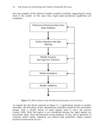
Selection of historical data from
plant database
Model validation
Outlier detection and data
filtering
Model structure
and regressor selection
Model estimation

Figure 3.1. Block scheme of the identification procedure of a soft sensor
As regards the first block reported in Figure 3.1, a preliminary remark is needed.
Generally, the first phase of any identification procedure should be the experiment
design, with a careful choice of input signals used to force the process
(Ljung, 1999). Here this aspect is not considered because the input signals are
necessarily taken from the historical system database. In fact, due to questions of
economy and/or safety, industries can seldom (and sometimes simply cannot)
perform measurement surveys.
Soft Sensor Design 29
This poses a number of challenging problems for the designer, such as:
missing data, collinearity, noise, poor representativeness of system dynamics (an
industrial system spends most of its time in steady state conditions and little
information on system dynamics can be extracted from data), etc.. A partial
solution to these problems is the careful investigation of very lengthy records (even
of several years) in order to find relevant data trends.
In this phase, the importance of interviews with plant experts and/or operators
cannot be stressed enough. In fact, they can give insight into relevant variables,
system order, delays, sampling time, operating range, nonlinearity, and so forth.

Without any expert help or physical insight, a soft sensor design can become an
unaffordable task and data can be only partially exploited.
Moreover, data collinearity and the presence of outliers need to be addressed by
applying adequate techniques, as will be shown in the following chapters of the
book.
Model structure is a set of candidate models among which the model should be
searched for. The model structure selection step is strongly influenced by the
purpose of the soft sensor design for a number of reasons. If a rough model is
required or the process works close to a steady state condition, a linear model can
be the most straightforward choice, due to the greater simplicity of the design
phase. A linear model can also be the correct choice when the soft sensor is to be
used to apply a classical control strategy. In all other cases a nonlinear model can
be the best choice to model industrial systems, which are very often nonlinear.
Other considerations about the dependence of the model structure on the
intended application have already been reported in Chapter 2.
Regressor selection is closely connected with the problem of model structure
selection. This aspect has been widely addressed in the literature in the case of
linear models. In this chapter, a number of methods that can be useful also for the
case of nonlinear models will be briefly described.
The same consideration holds true for model identification, consisting in
determining a set of parameters which will identify a particular model in the
selected class of candidates, on the basis of available data and suitable criteria. In
fact, approaches such as least mean square (LMS) based methodologies are widely
used for linear systems.
Though a corresponding well established set of theoretical results is not
available for nonlinear systems, methodologies like neural networks and
neuro-fuzzy systems are becoming standard tools, due to the good performance
obtained for a large number of real-world applications and the availability of
software tools that can help the designer.
In the applications described in this book we mainly use multi-layer perceptron

(MLP) neural networks. The topic of neural network design and learning is beyond
the scope of this book. Interested readers can refer to Haykin (1999).
The last step reported in Figure 3.1 is model validation. This is a fundamental
phase for data-driven models: a model that fits the data used for model
identification very well could give very poor results in simulations performed
using new sets of data. Moreover, models that look similar according to the set of
available data can behave very differently when new data are processed, i.e. during
a lengthy on-line validation phase.
30 Soft Sensors for Monitoring and Control of Industrial Processes
Criteria used for model validation generally depend on some kind of analysis
performed on model residuals and are different for linear and nonlinear models. A
number of validation criteria will be described later in this chapter and will be
applied to case studies in the following chapters.
Finally, it should be borne in mind that the procedure shown in Figure 3.1 is a
trial and error one, so that if a model fails the validation phase, the designer should
critically reconsider all aspects of the adopted design strategy and restart the
procedure trying different choices. This can require the designer going back to any
of the steps illustrated in Figure 3.1, and using all available insight until the success
of the validation phase indicates that the procedure can stop.
3.3 Data Selection and Filtering
The very first step in any model identification is the critical analysis of available
data from the plant database in order to select both candidate influential variables
and events carrying information about system dynamics, relevant to the intended
soft sensor objective. This task requires, of course, the cooperation of soft sensor
designer and plant experts, in the form of meetings and interviews. In any case, a
rule of thumb is that a candidate variable and/or data record can be eliminated
during the design process, so that it is better to be conservative during the initial
phase. In fact, if a variable carrying useful information is eliminated during this
preliminary phase, unsuccessful iteration of the design procedure in Figure 3.1 will
occur with a consequent waste of time and resources.

Data collection is a fundamental issue and the model designer might select data
that represent the whole system dynamic, when this is possible by running suitable
experiments on the plant. High-frequency disturbances should also be removed.
Moreover, careful investigation of the available data is required in order to
detect either missing data or outliers, due to faults in measuring or transmission
devices or to unusual disturbances. In particular, as in any data-driven procedure,
outliers can have an unwanted effect on model quality. Some of these aspects will
now be described in greater detail.
Data recorded in plant databases come from a sampling process of analog
signals, and plant technologists generally use conservative criteria in fixing the
sampling process characteristics. The availability of large memory resources leads
them to use a sampling time that is much shorter than that required to respect the
Shannon sampling theorem. In such cases, data resampling can be useful both to
avoid managing huge data sets and, even more important, to reduce data
collinearity.
A case when this condition can fail is when slow measuring devices are used to
measure a system variable, such as in the case of gas chromatographs or off-line
laboratory analysis. In such cases, static models are generally used. Nevertheless, a
dynamic MA or NMA model can be attempted, if input variables are sampled
correctly, by using the sparse available data over a large time span. Anyway, care
must be taken in the evaluation of model performance.
Digital data filtering is needed to remove high-frequency noise, offsets, and
seasonal effects.
Soft Sensor Design 31
Data in plant databases have different magnitudes, depending on the units
adopted and on the nature of the process. This can cause larger magnitude variables
to be dominant over smaller ones during the identification process. Data scaling is
therefore needed. Two common scaling methods are min–max normalization and
z-score normalization. Min–max normalization is given by:


xxx
xx
x
minminmax
minmax
minx
x
ccc




c
(3.1)
where:
x is the unscaled variable;
xƍ is the scaled variable;
min
x
is the minimum value of the unscaled variable;
max
x
is the maximum value of the unscaled variable;
min
x’
is the minimum value of the scaled variable;
max
x’
is the maximum value of the scaled variable.

The z-score normalization is given by:

x
x
meanx
x
V


c
(3.2)
where:
mean
x
is the estimation of the mean value of the unscaled variable;
ı
x
is the estimated standard deviation of the unscaled variable.
The z-score normalization is preferred when large outliers are suspected
because it is less sensitive to their presence.
Data collected in plant database are generally corrupted by the presence of
outliers, i.e. data inconsistent with the majority of recorded data, that can greatly
affect the performance of data-driven soft sensor design. Care should be taken
when applying the definition given above: unusual data can represent infrequent
yet important dynamics. So, after any automatic procedure has suggested a list of
outliers, careful screening of candidate outliers should be performed with the help
of a plant expert to avoid removing precious information. Data screening reduces
the risk of outlier masking, i.e. the case when an outlier is classified as a normal
sample, and of outlier swamping, i.e. the case when a valid sample is classified as
an outlier.

Outliers can either be isolated or appear in groups, even with regular timing.
Isolated outliers are generally interpolated, but interpolation is meaningless when
groups of consecutive outliers are detected. In such a case, they need to be
removed and the original data set should be divided into blocks to maintain the
correct time sequence among data, which is needed to correctly identify dynamic
models. Of course, this is not the case with static models, which require only the
corresponding samples for the remaining variables to be removed.
32 Soft Sensors for Monitoring and Control of Industrial Processes
The first step towards outlier filtering consists in identification of data
automatically labeled with some kind of invalidation tag (e.g. NaN,
Data_not_Valid, and Out_of_Range). After this procedure has been performed,
some kind of detection procedure can be applied. Though a generally accepted
criterion does not exist, a number of commonly used strategies will be described.
In particular, the following detection criteria will be addressed:
x 3
V
edit rule;
x Jolliffe parameters;
x residual analysis of linear regression.
In the 3
V
edit rule, the normalized distance d
i
of each sample from the
estimated mean is computed:

x
xi
i
meanx

d
V


(3.3)
and data are assumed to follow a normal distribution, so that the probability that
the absolute value of d
i
is greater than 3 is about 0.27% and an observation x
i
is
considered an outlier when |d
i
| is grater than this threshold.
To reduce the influence of multiple outliers in estimating the mean and
standard deviation of the variable, the mean can be replaced with the median and
the standard deviation with the median absolute deviation from the median (MAD).
The 3
V
edit rule with such a robust scaling is commonly referred to as the Hampel
identifier. Other robust approaches for outlier detection are reviewed in Chiang,
Perl and Seasholtz (2003).
The Jolliffe method, reviewed in Warne et al. (2004), is based on the use of the
following three parameters, named d
1i
2
, d
2i
2
, d

3i
2
, computed on the variables z,
obtained by applying either the principal component analysis (PCA) or projection
to latent structures (PLS) to the model variables. The parameters are computed as
follows:


¦


p
qpk
iki
zd
1
22
1
(3.4)

¦


p
qpk
k
ik
i
l
z

d
1
2
2
2
(3.5)

¦


p
qpk
kiki
lzd
1
22
3
(3.6)
where:
index i refers to the ith sample of the considered projected variable;