A general model of Fractional Frequency Reuse: Modelling and performance analysis
Bạn đang xem bản rút gọn của tài liệu. Xem và tải ngay bản đầy đủ của tài liệu tại đây (462.45 KB, 8 trang )
VNU Journal of Science: Comp. Science & Com. Eng, Vol. 36, No. 1 (2020) 38-45
Original Article
A General Model of Fractional Frequency Reuse:
Modelling and Performance Analysis
Lam Sinh Cong1,*, Nguyen Quoc Tuan1, Kumbesan Sandrasegaran2
1
Faculty of Electronics and Telecommunications, VNU University of Engineering and Technology,
Vietnam National University, Hanoi, 144 Xuan Thuy, Cau Giay, Hanoi, Vietnam
2
Faculty of Engineering and Information Technology, University of Technology Sydney, Australia
Received 01 November 2018
Revised 27 December 2018; Accepted 23 April 2019
Abstract: Fractional Frequency Reuse (FFR) is a promising to improve the spectrum e ciency in
the LongTerm Evolution (LTE) cellular network. In the literature, various research works have
been conducted to evaluate the performance of FFR. However, the presented analytical approach
only dealt with the special cases in which the users are divided into 2 groups and only two power
levels are utilised. In this paper, we consider a general case of FFR in which the users are
classified into groups and each group is assigned a serving power level. The mathematical model
of the general FFR is presented and analysed through a stochastic geometry approach. The derived
analytical results in terms of average coverage probability can covered all the related well-known
results in the literature.
Keywords: Fractional Frequency Reuse, LongTerm Evolution, coverage probability, stochastic geometry.
1. Introduction *
which represents 70% of the global population.
This will make mobile data traffic experience
eight-fold over the next five years. Therefore,
the requirement of spectral efficiency
improvement is a big challenge for the network
designers and operators.
One of the most popular to improve spectral
efficiency relates to frequency resource
allocation in which all Base Stations (BSs) are
allowed to operate on all Resource Blocks
(BSs). It is reminded that in Long Term
Evolution (LTE) network, each RB is defined
as having a time duration of 0.5ms and a
bandwidth of 180kHz made up of 12 sub-
In recent years, there has been a rapid rise
in the number of mobile users and mobile data
traffic. According to Cisco report [1], the
number of mobile users has a 5-fold growth
over the past 15 years. In 2015 more than a half
of a million devices have joined the cellular
networks. It is predicted that the number of
mobile users will reach 5.5 billion by 2020
_______
*
Corresponding author.
E-mail address:
/>
38
L.S. Cong et al. / VNU Journal of Science: Comp. Science & Com. Eng., Vol. 36, No. 1 (2020) 38-45
carriers with a sub-carrier spacing of 15kHZ.
Due to sharing RBs between BSs, InterCell
Interference (ICI) which is caused by using the
same RB at adjacent cells at the same time
becomes a main negative factor to limit
the network performance. Therefore, Fractional
Frequency Reuse (FFR) algorithms have
been introduced to control the reuse of
frequency [2].
The basic idea of FFR algorithm is to divide
the active users as well as the allocated RBs
into some groups so each group of users is
served by a specific group of RBs.
As recommendations of 3GPP [3,4,5], the BS
can utilise a lower power level to serve the user
with better wireless channel, a higher power level
to sever other users. By this way, the main
benefits are expected to achieve as follows:
• Reduce the power consumption of the
BSs. Some users with good communication
links such as low propagation path loss,
low fading can obtain their desired performance
with low power levels. Thus, the BSs do not
need to use high power levels to serve
those users.
• Improve system performance. It is
obvious that when a BS cuts its transmit power
off, its interfering power at the adjacent cell
will be reduced. Thus, the system performance
can be improved.
In the literature, there are a lot of research
works on modelling and performance analysis
of FFR in LTE networks by utilizing the
simulators such as [6,7,8,9,10] or stochastic
geometry models such as [11,12,13]. However,
these works only considered two groups of
users and thus only two power levels were
utilised. In a real network, the users as well as
RBs can be partitioned into more than two
groups. For example, a macro cell with radius
from 1 - 20 km can cover a huge area of up to
400 km2 . Thus, the users associated with that
macro cell experiences a wide range of SINR
and consequently they should be classified in
more than two groups to achieve better network
performance as well as save the power
consumption of BSs.
39
Hence in this paper, we consider the FFR
algorithm in which the users and RBs are
classified into groups ( 2 ). Thus, N
power levels are deployed, in which each user
group is served by a group of RB with a specific
power level. Figure 1 is an example of the
proposed model with frequency reuse = 3 .
Figure 1. A proposed FFR algorithm with = 3 .
The operational discipline of the system
model can be described as follows:
• Every = 3 cells use the same frequency
reuse pattern.
• The users are classified into 3 groups by
two SINR thresholds. There power levels are
denoted by P1 , P2 and P3 .
• The resource and power allocations are
presented in Table 1.
40
L.S. Cong et al. / VNU Journal of Science: Comp. Science & Com. Eng., Vol. 36, No. 1 (2020) 38-45
Table 1. Power allocation in the case of = 3
Cell 1
Cell 2
Cell 3
P2
P1
P3
P1
P3
RB group 1 P3
P2
RB group 3 P1
RB group 2
P2
In stead of assuming that there are only two
groups of users, we classified users into
groups by 1 SINR thresholds. The user j
is assigned to group j if its downlink SINR on
the control channel satisfy the following
condition
T j 1 < SINR < T j (3)
in which T j is the SINR threshold j , T0 = 0 ,
2. System model
T = , and T j 1 < T j for 0 < j .
We consider a single tier cellular network in
which the locations of BSs follows a spatial
Poison Point Process (PPP) with mean . The
user prefers a connection with the nearest BS.
According to 3GPP recommendations at
[4, 5], the operation of FFR includes two
phases, called establishment phase and
communication phase. The detail of these
phases are described as follows:
2.1. Establishment phase
The users measure and report the received
SINRs on the downlink control channels [4, 5]
for user classification purpose. Every BS is
continuously transmitting downlink control
information, and subsequently each control
channel experiences the ICI from all adjacent
BSs. Furthermore, since all BSs are assumed to
transmit on the control channels at the same
power, the ICI of the measured SINR during
this phase is given by.
I 0 = Pg r
j
( o )
j
j
(1)
gain and distance between BS j and the user,
respectively.
The reported SINR on the control channel is
given by
Pg ( o ) r
2 Pg (jo ) rj
We denote the transmit power used to serve
users in group j is Pj . Since the high power
levels are used to serve users with the lower
SINR on the control channel, Pj 1 < Pj for
1 < j N . We denote the ratio between the
power levels and the lowest power level P1 is
j = Pj /P1 . It is noted that the transmit power
Pj and j , (0 < j N ) are a constant
number.
Due to sharing the RBs between cells, each
user experiences ICI from all neighbouring
cells. The total ICI power at the typical user is
given by:
I = Pk g j rj (4)
k =1
jk
in which k is the set of interfering BSs
transmitting at Pj power level. The density of
)
where g (o
and r j are the channel power
j
SINR =
2.2. Communication phase
(2)
j
in which g and r is the channel power gain
and the distance from the user to its serving BS.
BSs in k is
.
Equation 4 can be considered as the general
case of the well-known FFR algorithm
modelling in the literature. For examples:
• When = 1 , Equation 4 degrades into
I = Pg j rj (5)
j
In Equation 5, consists of all adjacent
BSs. This equation has been found in the
literature such as [15, 16].
L.S. Cong et al. / VNU Journal of Science: Comp. Science & Com. Eng., Vol. 36, No. 1 (2020) 38-45
• When only two power levels are deployed
(only one SINR threshold is required): for
example group 1 is served by transmit power
P1 and 1 remaining groups are served by
transmit power P2 , Equation 4 degrades into
I = Pg
r
1
j1
j j
1
P2 g r
k =1 jk
j j
any BS in k ( j 1 ). Therefore, Equation 6 is
rewritten as
I = P1 g j rj P2 g j rj (7)
j1
j0
in which the density of BSs in 1 and 2 are
/ and ( 1)/ respectively.
Equation 7 is exactly the ICI of Soft FR.
The reported SINR on the data channel
during the communication phase is given by
SINR =
Pgr
P g r
k =1
Pc =
j k
P(T
n 1
< SINR < Tn )
n =1
It is reminded that the coverage probability
in Equation 9 is a function of random variables
such as channel power gain g , g j , distance
from the user to other BSs. Thus, to obtain the
average coverage probability of the typical user,
the expected value of Pc should be computed.
Therefore, the average coverage probability of
the user in the network is defined as following
equation:
P(Tˆ ) = E ( P(Tn1 < SINR < Tn )
n =1
in which g and r is the channel power
gain and the distance from the user to its
serving BS.
3 Performance evaluation
In this section, we derive the average
coverage probability of the typical user, which
can be classified into one of groups.
At a given time slot, the user at a distance
r from its serving BS is assigned to group j if
its downlink SINR satisfies Equation 3. The
corresponding
probability
is
P(Tn1 < SINR < Tn ) .
The user in group j is under the network
coverage if its SINR during the communication
phase, denoted by SINR , is greater than the
coverage threshold Tˆ . Thus, the coverage
probability is P( SINR > Tˆ ) .
(10)
P( SINRn > Tˆ ))
(8)
j j
(9)
P( SINR > Tˆ )
k
Therefore, the probability in which the
typical user is under the network coverage at a
given time slot is given by
(6)
Due to the thinning properties of PPP [16],
each BS in 1 is distributed independently to
41
Using the definition of SINR in Equation 2,
P(Tn1 < SINR < Tn )
g ( o ) r
= P Tn 1 <
<
T
n
g (jo ) rj
j
r
r
= P Tn 1 g (jo ) < g ( o ) < Tn g (jo )
rj
rj
j
j
= exp Tn 1 g (jo ) rj r
(a)
j
exp Tn g (jo ) rj r (11)
j
in which (a) due to g (o ) has a exponential
distribution.
Similarity, using the definition of SINR in
Equation 8, we have
P( SINR > Tˆ )
L.S. Cong et al. / VNU Journal of Science: Comp. Science & Com. Eng., Vol. 36, No. 1 (2020) 38-45
42
= P(
Pn gr
P g r
k
k =1
j k
Evaluating the fist element with notice that
> Tˆ )
k is a subset of , we divide into
independent subsets k with the densities of
BSs are / . Thus, the first element in
j j
P
= P g > Tˆ k g j rj r
k =1 Pn j k
(b )
P
= exp Tˆ k g j rj r (12)
Pn
k =1 jk
Equation 14 can be rewritten as follows:
where (b) due to g is a exponential random
variable.
Substituting Equations 11 and 12 into
Equation 10, the average coverage probability
P(Tˆ ) is given by
Pk
exp Tˆ g j rj r
Pn
k 1
j k
(
o
)
E
exp Tn 1 g j rj r
n 1
j
exp Tn g (jo ) rj r
j
(13)
Employing the properties of the Probability
Generating Function [19], we obtain
2
1
1
1
r dr
j j
r
Pk r
r
1Tn 1
1Tˆ
Pn r
r
j
j
E1 = E e
k =1
n =1
Using a change of variable y = (rj /r )2 , E1
can be rewritten as follows
Since all channel power gains are
independent exponential random variables
whose the Moment Generating Function (MGF)
1
, taking the expected
1 s
)
value of Equation with respect to g (o
and g j ,
j
is M X = E[e sx ] =
P(Tˆ ) is obtained by
1
1
E
P
r
r
n =1
k =1 jk
1 Tˆ k j 1 Tn 1
Pn rj
rj
1
1
E
P
r
r
n =1 k =1 j k
j
k
1 Tˆ
1 Tn
P
r
r
n j
j
1
1
E1 = E
k =1 j
Pk r
r
n =1
ˆ
k
1
T
1
T
n 1
Pn r j
rj
2
1
2 r 1 1
dy
Pk /2 1T y /2
1
ˆ
1
T
y
n 1
Pn
E1 = E e
n =1
k =1
Taking the expected value with respect to r ,
E1 is given by
2 re
n =1
0
r 2
e
r 2
k =1
ˆ
n (Tn 1 ,T , Pk )
dr
in which
(14)
1
1
dy
ˆ
n (Tn1 , T , Pk ) = 1
/2
1
P
ˆ k /2 1 Tn1 y
1 T P y
n
Similarly, the second element of Equation 14 is
given by
L.S. Cong et al. / VNU Journal of Science: Comp. Science & Com. Eng., Vol. 36, No. 1 (2020) 38-45
E2 = 2 re
n =1
r 2
0
r 2
ˆ
n (Tn ,T , Pk )
k =1
e
Equation 15 with T0 = 0 , T1 , Tm = m 2
dr
Substituting E1 and E2 into Equation 14 and
employing a change of variable in which
y = r 2 , the average coverage probability
P(Tˆ ) is given by:
P(Tˆ ) =
1
1
n (Tn1 , Tˆ , Pk )
k =1
1
(15)
1
n =1
ˆ
1 n (Tn , T , Pk )
k =1
Equation 15 provides the mathematical
expression of the average coverage probability
of the typical user in LTE network using FFR
with reuse factor in which users are
classified into user groups. This result can be
considered as the general form of the published
results in the literature. Take two special cases,
= 1 and = 3 , for example
Special case 1: = 1
In this case, T0 = 0 and T1 = , then
n =1
1
1
ˆ
n (0, T , Pk ) = 1
1
P
ˆ k /2
1 T P y
n
43
and Pm = Pn m, n > 2 , we obtain
1
P(Tˆ ) =
1
1
ˆ
ˆ
1 1 (0, T , P1 ) 1 (0, T , P1 )
1
1
1
ˆ
ˆ
1 2 (T1 , T , P1 ) 2 (T1 , T , P2 )
1
1
1
ˆ
ˆ
1 1 (T1 , T , P1 ) 1 (T1 , T , P2 )
(17)
The corresponding result for Soft Frequency
Reuse algorithm has been found in [17].
4 Simulation and discussion
dy
and n (, Tˆ , Pk ) = 0 .
The average coverage probability is given
by
P(Tˆ ) =
n =1
1
1 n (Tn 1 , Tˆ , Pk )
(16)
The expression in Equation 16 is the wellknown result on the average coverage
probability of the typical user in LTE network
with frequency reuse factor = 1 .
3.1 Special case 2: Only two power levels
are deployed
This model is usually called Soft Frequency
Reuse [18] in which the users and RBs are
divided into equal groups. Using the result in
Figure 2. Comparison between simulation and
analytical results.
Figure 2 presents the comparison between
the simulation and analytical results with
different values of path loss coefficient and
coverage threshold Tˆ .
The following parameters are selected for
simulation: the frequency reuse factor = 3 ,
the Rayleigh fading with a unit power, the
L.S. Cong et al. / VNU Journal of Science: Comp. Science & Com. Eng., Vol. 36, No. 1 (2020) 38-45
density of BSs = 0.025 ( BS/km2 ) and the
signal-to-noise ratio SNR = 10 dB.
As shown in Figure 2, the Monte Carlo
simulation results perfectly match with the
analytical results that can confirm the accuracy
of the analytical approach.
As indicated in Figure 2, the average
coverage probability of the typical user
increases with . This conclusion also has
been found in the literature and can be
explained as follows:
• Since the user is assumed to associate with
the nearest BS. The distance from the user to
the interfering BSs must be greater than that
from the user the serving BS.
• The path loss is proportional to the path
loss coefficient and the distance. Hence, when
the path loss exponent increases, the interfering
signals experience higher path loss than the
serving signal. In other words, SINR and
consequently average coverage probability
increase with the path loss exponent .
Figure 3 compares the average coverage
probability of the typical user with different
values of and SINR threshold. The selection
of parameters are as the following table:
T1
=2
=3
=4
Serving Power
of each group
T2
-10 (dB)
-10 (dB) 0 (dB)
-10 (dB) 0 (dB)
P1
T3
10 (dB)
P1/3
Table 2. Analytical parameters of Figure 3.
It is assumed that all users in Group 1 have
the same serving power and the users with high
SINRs will be served with lower transmit
powers. Thus, the serving power of the adjacent
group of users with high SINRs is reduced by 3
times. From Table 2, it is observed that the total
energy that is used by the BSs to serve the
associated users reduces with . For example,
the BSs in the case of = 2 will transmit at
two levels P1 and P1/3 to serve the associated
users. Meanwhile the BSs in the case of = 3
utilize P1 , P1/3 and P1/9 . Thus, it can be said
that the BSs in the case of = 2 consume
more energy than that in the case = 3 .
It is observed that the average coverage
probability reduces when increases. This
phenomenon is reasonable since the user
achieves the higher performance with high
serving power. However, in order to compare
the performance of frequency reuse algorithms,
various parameters and scenarios should be
considered [7].
0.8
0.75
Average Coverage Probability
44
0.7
0.65
=2
=3
=4
0.6
0.55
0.5
0.45
-10
-5
0
5
10
15
SINR Threshold
Figure 3. Comparison average coverage probability
with different values of .
5 Conclusion
In this paper, the general model of FFR in the
LTE network was modelled and analysed under
Rayleigh fading environment in which the BSs
are distributed according to a spatial Poisson
process. Instead of assuming that there are only
two power levels are used to serve the associated
user, this paper considered power levels in
which each power level is utilised to serve a
specific user group. The analytical results which
are verified by Monte Carlo simulation can be
considered as the general expressions of the
typical user performance since they contain all the
L.S. Cong et al. / VNU Journal of Science: Comp. Science & Com. Eng., Vol. 36, No. 1 (2020) 38-45
related results in the literature. For practical
perspective, based on the relationships between
frequency reuse factor , SINR threshold T j ,
density of BSs and the network performance that
were derived in the paper, the network designers
can select appropriate values to obtain the desired
user performance.
Acknowledgments
This work has been supported/partly
supported by VNU University of Engineering
and Technology under project number
CN18.01.
References
[1] Cisco, Cisco visual networking index: Global mobile
data traffic forecast update, 2015 - 2020, 2016.
[2] A.S. Hamza, S.S. Khalifa, H.S. Hamza, K.
Elsayed, A Survey on Inter-Cell Interference
Coordination Techniques in OFDMA-Based
Cellular Networks, IEEE Commun, Surveys &
Tutorials 15(4) (2013) 1642-1670
[3] 3GPP TR 36.819 V11.1.0, Coordinated multi-point
operation for LTE physical layer aspects, 2011.
[4] 3GPP Release 10 V0.2.1, LTE-Advanced (3GPP
Release 10 and beyond), 2014.
[5] 3GPP TS 36.211 V14.1.0, E-UTRA Physical
Channels and Modulation, 2016.
[6] R. Ghaffar, R. Knopp, Fractional frequency reuse
and interference suppression for ofdma networks,
in: 8th International Symposium on Modeling and
Optimization in Mobile, Ad Hoc and Wireless
Networks, 2010, pp. 273-277.
[7] Y. Kwon, O. Lee, J. Lee, M. Chung, Power
Control for Soft Fractional Frequency Reuse in
OFDMA System, Vol. 6018 of Lecture Notes in
Comput.Science, Springer Berlin Heidelberg,
2010, book section 7 (2010) 63-71.
[8] Enhancing LTE Cell-Edge Performance via
PDCCH ICIC, in: FUJITSU NETWORK
COMMUNICATIONS INC., 2011.
[9] A.S. Hamza, S.S. Khalifa, H.S. Hamza, K.
Elsayed, A Survey on Inter-Cell Interference
Coordination Techniques in OFDMA-Based
4
u
45
Cellular Networks, IEEE Commun, Surveys &
Tutorials
15(4)
(2013)
1642-1670.
/>
[10] A. Busson1, I. Lahsen-Cherif2, Impact of resource
blocks allocation strategies on downlink
interference and sir distributions in lte networks:
A stochastic geometry approach, Wireless
Communications and Mobile Computing.
[11] H. ElSawy, E. Hossain, M. Haenggi, Stochastic
Geometry for Modeling, Analysis and Design of
Multi-Tier and Cognitive Cellular Wireless
Networks: A Survey, IEEE Commun, Surveys
Tutorials
15(3)
(2013)
996-1019.
/>
[12] W. Bao, B. Liang, Stochastic Analysis of Uplink
Interference in Two-Tier Femtocell Networks:
Open Versus Closed Access, IEEE Trans,
Wireless Commun. 14(11) (2015) 6200-6215.
.
[13] H. Tabassum, Z. Dawy, E. Hossain, M.S. Alouini,
Interference Statistics and Capacity Analysis for
Uplink Transmission in Two-Tier Small Cell
Networks: A Geometric Probability Approach,
IEEE Trans, Wireless Commun 13(7) (2014)
3837-3852.
[14] J.G. Andrews, F. Baccelli, R.K. Ganti, A tractable
approach to coverage and rate in cellular networks,
IEEE Transactions on Communications 59(11)
(2011) 3122-3134.
[15] Y. Lin, W. Bao, W. Yu, B. Liang, Optimizing
User Association and Spectrum Allocation in
HetNets: A Utility Perspective, IEEE J. Sel. Areas
Commun.
33(6)
(2015)
1025-1039.
/>[16] M. Haenggi, Stochastic Geometry for Wireless
Networks, Cambridge Univ, Press, November 2012.
[17] H. ElSawy, E. Hossain, M. Haenggi, Stochastic
Geometry for Modeling, Analysis and Design of
Multi-Tier and Cognitive Cellular Wireless
Networks: A Survey, IEEE Commun, Surveys
Tutorials 15(3) (2013) 996-1019.
[18] Huawei, R1-050507: Soft Frequency Reuse
Scheme for UTRAN LTE, in: 3GPP TSG RAN
WG1 Meeting #41, 2005.
[19] M.A. Stegun, I.A., Handbook of Mathematical
Functions
with
Formulas,
Graphs
and
Mathematical Tables, 9th Edition, Dover
Publications, 1972.