Atomistically kinetic simulations of carbon diffusion in ɑ iron with point defects001
Bạn đang xem bản rút gọn của tài liệu. Xem và tải ngay bản đầy đủ của tài liệu tại đây (7.48 MB, 91 trang )
VIETNAM NATIONAL UNIVERSITY, HANOI
VIETNAM JAPAN UNIVERSITY
HO NGOC NAM
ATOMISTICALLY KINEMATIC
SIMULATIONS OF CARBON DIFFUSION
IN α-IRON WITH POINT DEFECTS
MASTER’S THESIS
Hanoi, 2019
VIETNAM NATIONAL UNIVERSITY, HANOI
VIETNAM JAPAN UNIVERSITY
HO NGOC NAM
ATOMISTICALLY KINEMATIC
SIMULATIONS OF CARBON DIFFUSION
IN α-IRON WITH POINT DEFECTS
MAJOR: NANOTECHNOLOGY
CODE: PILOT
RESEARCH SUPERVISORS:
Prof. Dr. YOJI SHIBUTANI
Dr. NGUYEN TIEN QUANG
Hanoi, 2019
ACKNOWLEDGMENT
To accomplish this thesis, I have received great support, helpful advice, and
guidance from respectful professors, lecturers, researchers, and staff in Vietnam
Japan University and Osaka University.
I would like to express my gratefulness to my supervisors, Prof. Dr. Yoji Shibutani
and Dr. Nguyen Tien Quang for supplying great researching environments in
laboratories, and for giving helpful instructions, guidance, advice, and inspirations
during my master course.
Finally, I am thankful to my family for the support, companion, and mobilization,
which is an essential element for me to finish the thesis.
Hanoi, 10 June 2019
Student
HO NGOC NAM
TABLE OF CONTENTS
ACKNOWLEDGMENT............................................................................................ i
LIST OF FIGURES.................................................................................................... i
LIST OF TABLES...................................................................................................iii
LIST OF ABBREVIATIONS................................................................................... iv
CHAPTER 1. INTRODUCTION.............................................................................. 1
CHAPTER 2. THEORETICAL BASICS.................................................................. 6
CHAPTER 3. RESULTS AND DISCUSSION....................................................... 21
CONCLUSION....................................................................................................... 54
FUTURE PLAN...................................................................................................... 55
LIST OF PUBLISCATIONS................................................................................... 56
REFFRENCES........................................................................................................ 57
APPENDIX............................................................................................................. 63
LIST OF FIGURES
Figure 1.1. The relation between elongation (ductility) and tensile strength in low
carbon steel for general applications [4] .....................................................................
Figure 1.2. Phase diagram of iron-carbon alloy by different carbon content [19]. ....
Figure 1.3. Simulation picture of typical defects in iron-carbon alloy ......................
Figure 2.1. Reaction energy diagram as a function of reaction coordinate q
isomerization reaction [37]. ........................................................................................
Figure 2.2. Illustration of finding the minimum energy path by NEB. Each image
on the chain of the system is connected by spring forces which located along the
minimum energy line between two minimum energy points [44]. ...........................
Figure 2.3. Decomposition of force on an image [38]. ............................................
Figure 2.4. Contour plot of the potential energy surface for an energy-barrierlimited infrequent-event system. After many vibrational periods, the trajectory finds a
way out of the initial basin, passing a ridgetop into a new state. The dots indicate
saddle points [45]. .....................................................................................................
Figure 2.5 the transition of atom when diffusing from the state (i) to the state (j) by
crossing the energy barrier
Figure 2.6 The K-th transition is chosen because its assigned value of s(K)
intercepts r2
i
[44]. ...................................................................................................
Figure 3.1 Positions 1, 2 of carbon correspond to O site, and 3 corresponds to T site
...................................................................................................................................
Figure 3.2: Positions carbon is adopted in iron system ...........................................
Figure 3.3. Configurations of BCC iron structure in case of two carbons. ..............
Figure 3.4: Configurations of BCC iron structure in case of three carbons. ............
Figure 3.5: Configurations of BCC iron structure in case four carbons ..................
Figure 3.6. Energy landscape (a, b) and energy contour line (c, d) of iron-carbon
system in case of vacancy/without vacancy is created by [010] and [001] directions.
...................................................................................................................................
Figure 3.7: The change position and angle of iron atoms around carbon atom,
which is doped between two iron atoms lead to relaxing configuration. ..................
Figure 3.8 Binding energy of carbon-vacancy is calculated by DFT calculation and
MD method in case 1V-1C. ......................................................................................
Figure 3.9: Configuration 3 after optimized in case 2 carbon atoms .......................
Figure 3.10. Configuration 3 after optimized ...........................................................
Figure 3.11. The most stable configuration in case 4 carbon atoms in iron ............
i
Figure 3.12. Trapping energy is calculated in two ways: “sequential” way (blue
line) and “simultaneous” way (red line).................................................................. 38
Figure 3.13. Minimum energy paths of carbon in case 1C by two possible ways. .. 39
nd
Figure 3.14. Eight diffusion paths of 2 carbon around vacancy in case of 2 carbon
atoms....................................................................................................................... 41
Figure 3.15. Minimum energy paths of carbon in case 2C..................................... 42
rd
Figure 3.16. Seven diffusion paths of the 3 carbon atom around the vacancy in
case of 3 carbon atoms............................................................................................ 45
Figure 3.17. Minimum energy paths of carbon in case 3C..................................... 46
Figure 3.18. Jumping rate in case of 1, 2 and 3 carbon atoms as an inverse function
of temperature......................................................................................................... 50
Figure 3.19. Diffusion coefficient vs. temperature in 2 cases: perfect case and
vacancy case............................................................................................................ 53
ii
LIST OF TABLES
Table 1.1. Different phases of steel based on carbon content [23]............................3
Table 3.1. Configuration of system when carbon is adopted in position 1, 2, 3......29
Table 3.2. The binding energy between vacancy-carbon at position P1 to P7 for
both size 3x3x3/8x8x8 was calculated with the consideration of the distance........32
Table 3.3. Binding energy at P1 by DFT method from some authors is collected for
system size 3x3x3 and 4x4x4.................................................................................. 32
Table 3.4: Binding energy from MD and DFT method (for size 3x3x3) is computed
for seven configurations.......................................................................................... 34
Table 3.5. Position of carbon atoms before and after optimized.............................35
Table 3.6. The binding energy of seven configurations in case of 4 carbons..........35
Table 3.7: Position of carbon atoms before and after optimized in case 3C...........36
Table 3.8: Binding energy of 7 configurations in case 4 carbon atoms...................37
Table 3.9: The change position of 4 carbon in configuration 4 after optimized......37
Table 3.10. Relaxation configurations in two carbon case...................................... 43
Table 3.11. Comparison between two durable configurations of two carbon atoms
in perfect and vacancy case..................................................................................... 44
Table 3.12. Relaxation configurations in three carbon case....................................47
Table 3.13. Comparison between two stable configurations of three carbon atoms in
perfect and vacancy case......................................................................................... 48
Table 3.14. Mean square displacement of carbon atom vs time of some
temperatures in both case: perfect case and vacancy case by kMC.........................52
iii
LIST OF ABBREVIATIONS
Abbreviation
Description
ABOP
Analytic Bond-order Potential
BCC
Body-Centered Cubic
DFT
Density Functional Theory
MD
Molecular Dynamics
MEP
Minimum energy path
kMC
Kinetic Monte Carlo
FDM
Finite Different Method
CI-NEB
Climbing image – Nudged Elastic Band
O-site
Octahedral site
T-site
Tetragonal site
TST
Transition State Theory
LAMMPS
Large-scale Atomic/Molecular Massively Parallel
Simulator
iv
CHAPTER 1. INTRODUCTION
Nowadays, along with the steady development of science and technology, the
achievements in scientific research are increasingly contributing to society,
especially in the field of nanotechnology. Research, development, and application of
potential and unique properties from nanoscale materials have brought many
improvements and breakthroughs compared to previous traditional materials [15].
The field of computational materials science is considered as one of the areas of top
concern in material science today [9]. Calculations are implemented based on the
theoretical foundations, which apply to specific subjects under the simulation
process supported by modern computer systems, acting as useful tools in describing,
verifying, predicting the rules, physical phenomena occurring inside objects and
between objects. The development process of computational science is an essential
and inseparable part of the practical application in industry. In particular, the
calculation related to iron-carbon alloys is a good example and plays a crucial role in
the development of the steel industry.
Until now, the steel industry has an extraordinary development, which can be divided
into three main generations. The first generation - Conventional low carbon steels can
be mentioned as high strength low-alloy products (HSLA) steels, advanced high
strength steels (AHSS), IF (Interstitial Free), DP (Dual Phase) or so-called TRIP /
TWIP (Transformation or Twinning Induced Plasticity), etc. is incredibly famous and
widely used steel generation today [4]. The second generation - Austenitic-Based Steels
has been developed, and the third generation is still being researched and developed.
For different generations, superiorities and disadvantages still exist not only on
mechanical properties but also on product costs. Therefore, the main goal of this thirdgeneration material system is to continue to improve the desired mechanical
1
properties while cutting the costs and enhancing the connectivity of materials
compared to previous generations.
Figure 1.1. The relation between elongation (ductility) and tensile strength in low
carbon steel for general applications [4]
Overview of iron-carbon alloy
With its long history of development, steel is still one of the most widely used
materials in our modern world [24], and it can be seen that steel is present in most
buildings from small houses to skyscrapers, roads, and bridges. The reason for this
material becoming popular and preferable comes from its characteristics. The
versatility, durability, and strength of steel can meet requirements as well as
applications for a variety of purposes, and it is also an affordable and
environmentally friendly option [5]. Research on steel is still an exciting field that
scientists, especially in material science, are interested in improving the properties
of this traditional material.
2
Figure 1.2. Phase diagram of iron-carbon alloy by different carbon content [19].
Table 1.1. Different phases of steel based on carbon content [23].
Phase
-Fe
- Fe
δ - Fe
Fe3C
Fe-C solid
solution
3
Based on the structure of pure iron and steel, it is easy to see that these are similar
structural materials. The most significant and vital difference comes from the
occurrence of carbon impurity concentrations in the system. More specifically,
when the carbon concentration in the alloy of iron exceeds the 2.1wt% threshold,
the alloy is considered as cast iron, which is very hard and also very brittle. In the
case of carbon concentration less than 0.08wt%, it becomes softer when compared
to cast iron, but its ability as incurvation or distortion was better without breaking,
which is necessary to play a role as a structural steel in the building. When carbon
concentration is between 0.2wt% and 2wt%, the properties of steel become special
thanks to the balance between hardness and ductility [36]. However, how to control
both level and location of carbon in iron is the most challenging problem we faced.
So, there is no denying that the history of the steel industry is defined based on
carbon concentration control techniques.
The appearance of carbon atoms in the iron system even in small quantities is still
thought to have a significant effect based on the energy and kinetic properties of the
system. It can be seen that carbide formation comes from exceeding the limit of
carbon solubility, which contributes significantly to improving the durability and
hardness of metals as in steel. On the opposite side, when the carbon concentration
in the system is below the solubility limit, the thermal and mechanical properties of
the system can change significantly only by a minimal amount of carbon atoms
(several tens of ppm) in interstitial sites or when they interact strongly with defects
in steel [27].
The purpose and objectives of research
The real lattice is not perfect but contains many types of defects, which can be
referred to as vacancy, dislocation, or grain boundary [41]. While vacancy is well
known as a typical case of point defect and also a simple case which we can
consider. Study about the vacancy case in BCC structure of iron will help us
understand clearly about the role and the effects of vacancy to the diffusion and
clustering of carbon in iron matrix.
4
Figure 1.3. Simulation picture of typical defects in iron-carbon alloy
The cause of the interaction between carbon and metals has a tremendous scientific and
technological interest which has essential effects on the yield stress and the subconsequent mechanical properties and also a broad range of implications in the scope of
material science [26]. Research on atomic carbon concentration dissolved in iron as
well as its distribution and diffusion in iron plays a vital role in making a view insight
of phenomena such as carbide precipitation, martensite aging, and ferrite
transformation [31]. The restriction of system size when calculating using First
principle method causes Molecular Dynamic (MD) to be a reasonable substitute for
large systems [39]. However, the accuracy of MD simulations largely depends on the
choice of interatomic potential. Recently, Nguyen et al. [31] developed a new
interatomic potential to describe the interaction of Fe-C system based on the analytic
bond-order potential (ABOP) formalism [29], which gives good results in describing
minimum energy path (MEP) of carbon with T site found as a transition point [25].
This topic is intended to provide a clearer and more objective view of the point
defect in the iron-carbon alloy as well as its effect on the diffusion process of carbon
impurities in the alpha iron system through the use of atomistically kinematic
simulations.
5
CHAPTER 2. THEORETICAL BASICS
The transition state theory
Transition state theory is a theoretical method used to predict the rate of chemical
reactions. The theory was proposed by Erying and Polanyi in 1935 to explain the
bipolar reactions based on the relationship between kinetics and thermodynamics.
This theory is based on the initial assumption that the reaction speed can be
calculated completely, so it is also called the theory of absolute reaction speed [1].
In particular, if there is only one barrier between the reactant and the product, the
transition state theory specifies how to calculate the reaction rate constant. The
transitional state theory assumes the validity of only one condition, but a significant
condition, namely on one side of the barrier, the states of the system in equilibrium.
If there is only one barrier between reactants and products, then the reactant should
be kept in equilibrium. The simplicity of the transition state theory is lost if the
reactants are selected according to the state. The assumption of statistics given by
the transitional state theory is not about the dynamics of the reaction; instead, it is
about the balanced nature of the reactants placed on one side of the barrier. One
fundamental meaning of this assumption is that it allows theory to be cast in
anatomical terms. The statistical assumption given by transitional state theory is a
specification of reactants that theory can be applied.
The basic foundation for this theory can be understood as being based on the ability to
activate the internal bonds of a molecule. In other words, the reaction only occurs when
the activation energy is high enough for it to overcome the activation barrier. When the
activation energy required for the reaction is higher than that of the thermal
energy supplied, k T then the probability of activating a molecule is very low. In B
order to provide more energy for the reaction, more collisions occur as a significant
event for the reaction. When a molecule is activated, the probability for it to cross the
energy barrier becomes more accessible and faster. In which the constant representing
the speed of the reaction is determined as (k BT / h )K # , with (k BT / h ) being the rate
6
of a molecule when it passes through the barrier and
of activated complexes.
K
is the equilibrium constant
The transition state or activated complex can be assumed to have all the attributes of a
typical molecule except that one of the vibrational degrees of freedom is converted into
a translation degree of freedom along with the reaction coordinates. The reaction is
thought to proceed through an activated complex, the transition state, located at an
energy barrier separating reactants and products. It can be visualized by the travel over
a potential energy surface, such as a mountain landscape where the barrier lies at the
saddle point, the mountain pass or col. The event is described by one degree of
freedom (e.g.,
coordinate,
q
For an isomerization reaction, a representation of the potential energy dependence of
the reaction on reaction coordinate
is defined by
Where Eb is activation energy (the energy at qb
overall reaction energy
reactant.
Figure 2.1. Reaction energy diagram as a function of reaction coordinate q for an
isomerization reaction [37].
7
As mentioned by the TST, the activation complex or transition state is considered to
be in equilibrium with reactant molecules; the rate of reaction is equal to the number
of activation complexes which pass over the product side per unit time. The
transition-state expression for the rate of reaction is described as below:
k
(2.1)
TST
Where
kB
is the Boltzmann c
#
and K
The constant equilibrium K
the relation.
where
equal
G
#
product of the temperature times the entropy of the system in their standard states.
G
Substituting the value of G#
(2.3)
in (2.3):
Then, the expression for the rate constant of a reaction on the basic of TST is shown
below
Where
H
The goal of transitional state theory is to predict the rate of a reaction on a known
potential energy surface. The potential energy surface is, in general, a high
dimensional surface, but usually, a large number of degrees of freedom (such as the
8
orientation of molecules) can be neglected. Ideally, one would like to project the
potential energy surface onto a single dimension, which is called the reaction
coordinate. The reaction coordinate can be as simple as the distance between two
molecules. One of the accomplishments of transition state theory is the theoretical
justification of the Arrhenius law, which was proposed by Svante August Arrhenius
in 1889 that the effective attempt frequency
as [13]:
k
(2.7)
#
where
i
the saddle point, where one of the vibration frequencies should be
i
imaginary
frequency.
From that, the rate of each event will be defined as the following:
(2.8)
k
is the activation energy, k is the Boltzmann factor, T is the temperature.
Where E
d
2.2. Nudged Elastic Band Method
In energy surface analysis, it is known that finding the minimum energy path between
two minimum energy points becomes an important problem for determining the diffuse
properties of atoms in the matrix. Until now, the Nudged Elastic Band method (NEB) is
still the most advanced method for determining minimum energy paths [22]. The basic
idea of this method comes from creating a series of replicas (or images) between two
minimum energy points, from which the replicas are linked together to form a chain
bonded by fictitious spring force. Finally, the actual minimum energy
9
path will be revealed when the total energy of the string of replicas is minimized by
a suitable algorithm. NEB method can be used for:
➢
➢
➢
Chemical reactions on surface;
Diffusion processes;
Phase transformations, etc.
A modified version based on the NEB method is Climbing Image- Nudged Elastic
Band (CI-NEB). After minimizing the energy of all the replicas together based on
the virtual elastic force, the appropriate algorithm will be used to push the highest
energy image from another up to the saddle point by maximizing its energy along
the direction defined by the band [44]. In this way, the CI-NEB method not only
helps to determine a saddle point more accurately but also provides an overview of
the minimum energy line shape, which also allows us to identify more than a saddle
point along with the atomic movement of the atom. Therefore, it has helped to give
us a more precise view as well as providing the necessary parameters for calculating
the diffusion properties of atoms.
Figure 2.2. Illustration of finding the minimum energy path by NEB. Each image
on the chain of the system is connected by spring forces which located along the
minimum energy line between two minimum energy points [44].
10
Figure 2.3. Decomposition of force on an image [38].
By a force projection scheme in which potential forces act perpendicular to the band
and spring forces act along the band, the images along the NEB are relaxed to the
MEP. The process is carried out through the following formulas [38]:
Spring force on each image is given by:
(2.9)
F
i
To find MEP, we need to minimize the following objective function:
S ( r (0) , r (1) ,..., r (M) = V ( r (i) ) +
After that, the total force on the image is considered as:
F=−V(r)+F
(2.11)
i
Projecting the component of the total force perpendicular to the reaction pathway
out of the total force:
Fi EB = − Vi ⊥ + Fi S
11
=− V −
(2.12)
i
Removes perpendicular component of spring force:
(2.13)
=− V −
i
The saddle point is exceptionally crucial for characterizing the transition state
within harmonic transition state theory (HTST). The difference between the saddle
point energy and that of the initial state determines the exponential term in the
Arrhenius rate, and the MEP can be obtained by minimizing from the saddle
point(s). An efficient approach for seeking a saddle between known states is to use
the Climbing Image - NEB (CI-NEB) method [43]. In this method, the highest
energy image feels no spring forces and climbs to the saddle via a reflection in the
force along the tangent [20], [21], [30].
The force at the max-energy image without spring forces:
FMAXNEB = − VMAX
Kinetic Monte Carlo method
The kinetic Monte Carlo (kMC) is a simulation method intended to simulate the time
evolution of some processes occurring in nature [8]. Typically, these are processes that
occur with known transition rates among states. It is important to understand that these
rates are inputs to the kMC algorithm, the method itself cannot predict them [7].
The kinetic Monte Carlo method provides a simple yet powerful and flexible tool for
exercising the concerted action of fundamental, stochastic, physical mechanisms to
create a model of the phenomena that they produce. By using kMC method, we can
12