The Binomial Distribution
Bạn đang xem bản rút gọn của tài liệu. Xem và tải ngay bản đầy đủ của tài liệu tại đây (2.93 MB, 17 trang )
7
CHAPTER
The Binomial
Distribution
Introduction
Many probability problems involve assigning probabilities to the outcomes
of a probability experiment. These probabilities and the corresponding
outcomes make up a probability distribution. There are many different
probability distributions. One special probability distribution is called the
binomial distribution. The binomial distribution has many uses such as in
gambling, in inspecting parts, and in other areas.
114
Copyright © 2005 by The McGraw-Hill Companies, Inc. Click here for terms of use.
Discrete Probability Distributions
In mathematics, a variable can assume different values. For example, if one
records the temperature outside every hour for a 24-hour period, temperature
is considered a variable since it assumes different values. Variables whose
values are due to chance are called random variables. When a die is rolled, the
value of the spots on the face up occurs by chance; hence, the number of
spots on the face up on the die is considered to be a random variable. The
outcomes of a die are 1, 2, 3, 4, 5, and 6, and the probability of each outcome
occurring is
1
6
. The outcomes and their corresponding probabilities can be
written in a table, as shown, and make up what is called a probability
distribution.
Value, x 123456
Probability, P(x)
1
6
1
6
1
6
1
6
1
6
1
6
A probability distribution consists of the values of a random variable and
their corresponding probabilities.
There are two kinds of probability distributions. They are discrete and
continuous.Adiscrete variable has a countable number of values (countable
means values of zero, one, two, three, etc.). For example, when four coins are
tossed, the outcomes for the number of heads obtained are zero, one, two,
three, and four. When a single die is rolled, the outcomes are one, two, three,
four, five, and six. These are examples of discrete variables.
A continuous variable has an infinite number of values between any two
values. Continuous variables are measured. For example, temperature is a
continuous variable since the variable can assume any value between 108 and
208 or any other two temperatures or values for that matter. Height and
weight are continuous variables. Of course, we are limited by our measuring
devices and values of continuous variables are usually ‘‘rounded off.’’
EXAMPLE: Construct a discrete probability distribution for the number of
heads when three coins are tossed.
SOLUTION:
Recall that the sample space for tossing three coins is
TTT, TTH, THT, HTT, HHT, HTH, THH, and HHH.
CHAPTER 7 The Binomial Distribution
115
The outcomes can be arranged according to the number of heads, as
shown.
0 heads TTT
1 head TTH, THT, HTT
2 heads THH, HTH, HHT
3 heads HHH
Finally, the outcomes and corresponding probabilities can be written in a
table, as shown.
Outcome, x 0123
Probability, P(x)
1
8
3
8
3
8
1
8
The sum of the probabilities of a probability distribution must be 1.
A discrete probability distribution can also be shown graphically by
labeling the x axis with the values of the outcomes and letting the values on
the y axis represent the probabilities for the outcomes. The graph for the
discrete probability distribution of the number of heads occurring when three
coins are tossed is shown in Figure 7-1.
There are many kinds of discrete probability distributions; however, the
distribution of the number of heads when three coins are tossed is a special
kind of distribution called a binomial distribution.
Fig. 7-1.
CHAPTER 7 The Binomial Distribution
116
A binomial distribution is obtained from a probability experiment called a
binomial experiment. The experiment must satisfy these conditions:
1. Each trial can have only two outcomes or outcomes that can be
reduced to two outcomes. The outcomes are usually considered as a
success or a failure.
2. There is a fixed number of trials.
3. The outcomes of each trial are independent of each other.
4. The probability of a success must remain the same for each trial.
EXAMPLE: Explain why the probability experiment of tossing three coins is
a binomial experiment.
SOLUTION:
In order to be a binomial experiment, the probability experiment must satisfy
the four conditions explained previously.
1. There are only two outcomes for each trial, head and tail. Depending
on the situation, either heads or tails can be defined as a success and
the other as a failure.
2. There is a fixed number of trials. In this case, there are three trials
since three coins are tossed or one coin is tossed three times.
3. The outcomes are independent since tossing one coin does not
effect the outcome of the other two tosses.
4. The probability of a success (say heads) is
1
2
and it does not change.
Hence the experiment meets the conditions of a binomial experiment.
Now consider rolling a die. Since there are six outcomes, it cannot be
considered a binomial experiment. However, it can be made into a binomial
experiment by considering the outcome of getting five spots (for example) a
success and every other outcome a failure.
In order to determine the probability of a success for a single trial of a
probability experiment, the following formula can be used.
n
C
x
ÁðpÞ
x
Áð1 À pÞ
nÀx
where n ¼ the total number of trials
x ¼ the number of successes (1, 2, 3, ..., n)
p ¼ the probability of a success
The formula has three parts:
n
C
x
determines the number of ways a success
can occur. ( p)
x
is the probability of getting x successes, and (1 À p)
nÀx
is the
probability of getting n À x failures.
CHAPTER 7 The Binomial Distribution
117
EXAMPLE: A coin is tossed 3 times. Find the probability of getting two
heads and a tail in any given order.
SOLUTION:
Since the coin is tossed 3 times, n ¼ 3. The probability of getting a head (suc-
cess) is
1
2
,sop ¼
1
2
and the probability of getting a tail (failure) is 1 À
1
2
¼
1
2
;
x ¼ 2 since the problem asks for 2 heads. (n À x) ¼ 3 À 2 ¼ 1.
Hence,
Pð2 headsÞ¼
3
C
2
Á
1
2
2
1
2
1
¼ 3 Á
1
4
1
2
¼
3
8
Notice that there were
3
C
2
or 3 ways to get two heads and a tail. The
answer
3
8
is also the same as the answer obtained using classical probability
that was shown in the first example in this chapter.
EXAMPLE: A die is rolled 3 times; find the probability of getting exactly
one five.
SOLUTION:
Since we are rolling a die 3 times, n ¼ 3. The probability of getting a 5 is
1
6
.
The probability of not getting a 5 is 1 À
1
6
or
5
6
. Since a success is getting
one five, x ¼ 1 and n À x ¼ 3 À 1 ¼ 2.
Hence,
Pðone 5Þ¼
3
C
1
Á
1
6
1
Á
5
6
2
¼ 3 Á
1
6
Á
25
36
¼
25
72
or 0:3472
About 35% of the time, exactly one 5 will occur.
CHAPTER 7 The Binomial Distribution
118
EXAMPLE: An archer hits the bull’s eye 80% of the time. If he shoots
5 arrows, find the probability that he will get 4 bull’s eyes.
SOLUTION:
n ¼ 5, x ¼ 4, p ¼ 0.8, 1 À p ¼ 1 À 0.8 ¼ 0.2
Pð4 bull’s eyesÞ¼
5
C
4
ð0:8Þ
4
ð0:2Þ
1
¼ 5 Á 0:08192
¼ 0:4096
In order to construct a probability distribution, the following formula
is used:
n
C
x
p
x
(1 À p)
n À x
where x ¼ 1, 2, 3, ...n.
The next example shows how to use the formula.
EXAMPLE: A die is rolled 3 times. Construct a probability distribution for
the number of fives that will occur.
SOLUTION:
In this case, the die is tossed 3 times, so n ¼ 3. The probability of getting a 5
on a die is
1
6
, and one can get x ¼ 0, 1, 2, or 3 fives.
For x ¼ 0,
3
C
0
1
6
0
5
6
3
¼ 0:5787
For x ¼ 1,
3
C
1
1
6
1
5
6
2
¼ 0:3472
For x ¼ 2,
3
C
2
1
6
2
5
6
1
¼ 0:0694
For x ¼ 3,
3
C
3
1
6
3
5
6
0
¼ 0:0046
Hence, the probability distribution is
Number of fives, x 0123
Probability, P(x) 0.5787 0.3472 0.0694 0.0046
CHAPTER 7 The Binomial Distribution
119