The Normal Distribution

CHAPTER
9
The Normal
Distribution
Introduction
A branch of mathematics that uses probability is called statistics. Statistics is
the branch of mathematics that uses observations and measurements called
data to analyze, summarize, make inferences, and draw conclusions based on
the data gathered. This chapter will explain some basic concepts of statistics
such as measures of average and measures of variation. Finally, the
relationship between probability and normal distribution will be explained
in the last two sections.
147
Copyright © 2005 by The McGraw-Hill Companies, Inc. Click here for terms of use.
Measures of Average
There are three statistical measures that are commonly used for average.
They are the mean, median, and mode. The mean is found by adding the data
values and dividing by the number of values.
EXAMPLE: Find the mean of 18, 24, 16, 15, and 12.
SOLUTION:
Add the values: 18 þ 24 þ 16 þ 15 þ 12 ¼ 85
Divide by the number of values, 5: 85 Ä 5 ¼ 17
Hence the mean is 17.
EXAMPLE: The ages of 6 executives are 48, 56, 42, 52, 53 and 52. Find the
mean.
SOLUTION:
Add: 48 þ 56 þ 42 þ 52 þ 53 þ 52 ¼ 303
Divide by 6: 303 Ä 6 ¼ 50.5
Hence the mean age is 50.5.
The median is the middle data value if there is an odd number of data
values or the number halfway between the two data values at the center, if

there is an even number of data values, when the data values are arranged in
order.
EXAMPLE: Find the median of 18, 24, 16, 15, and 12.
SOLUTION:
Arrange the data in order: 12, 15, 16, 18, 24
Find the middle value: 12, 15,
16, 18, 24
The median is 16.
EXAMPLE: Find the median of the number of minutes 10 people had to wait
in a checkout line at a local supermarket: 3, 0, 8, 2, 5, 6, 1, 4, 1, and 0.
SOLUTION:
Arrange the data in order: 0, 0, 1, 1, 2, 3, 4, 5, 6, 8
The middle falls between 2 and 3; hence, the median is (2 þ 3) Ä 2 ¼ 2.5.
CHAPTER 9 The Normal Distribution
148
The third measure of average is called the mode. The mode is the data value
that occurs most frequently.
EXAMPLE: Find the mode for 22, 27, 30, 42, 16, 30, and 18.
SOLUTION:
Since 30 occurs twice and more frequently than any other value, the mode
is 30.
EXAMPLE: Find the mode for 2, 3, 3, 3, 4, 4, 6, 6, 6, 8, 9, and 10.
SOLUTION:
In this example, 3 and 6 occur most often; hence, 3 and 6 are used as the
mode. In this case, we say that the distribution is bimodal.
EXAMPLE: Find the mode for 18, 24, 16, 15, and 12.
SOLUTION:
Since no value occurs more than any other value, there is no mode.
A distribution can have one mode, more than one mode, or no mode.
Also, the mean, median, and mode for a set of values most often differ

somewhat.
PRACTICE
1. Find the mean, median, and mode for the number of sick days nine
employees used last year. The data are 3, 6, 8, 2, 0, 5, 7, 8, and 5.
2. Find the mean, median, and mode for the number of rooms seven
hotels in a large city have. The data are 332, 256, 300, 275, 216, 314,
and 192.
3. Find the mean, median, and mode for the number of tornadoes that
occurred in a specific state over the last 5 years. The data are
18, 6, 3, 9, and 10.
4. Find the mean, median, and mode for the number of items 9 people
purchased at the express checkout register. The data are
12, 8, 6, 1, 5, 4, 6, 2, and 6.
5. Find the mean, median, and mode for the ages of 10 children who
participated in a field trip to the zoo. The ages are 7, 12, 11, 11, 5,
8, 11, 7, 8, and 6.
CHAPTER 9 The Normal Distribution
149
ANSWERS
1. Mean ¼
3 þ 6 þ 8 þ 2 þ 0 þ 5 þ 7 þ 8 þ 5
0
¼
44
9
¼ 4:89
Median ¼ 5
Mode ¼ 5 and 8
2. Mean ¼
332 þ 256 þ 300 þ 275 þ 216 þ 314 þ 192

7
¼
1885
7
¼ 269:29
Median ¼ 275
Mode ¼ None
3. Mean ¼
18 þ 6 þ 3 þ 9 þ 10
5
¼
46
5
¼ 9:2
Median ¼ 9
Mode ¼ None
4. Mean ¼
12 þ 8 þ 6 þ 1 þ 5 þ 4 þ 6 þ 2 þ 6
9
¼
50
9
¼ 5:56
Median ¼ 6
Mode ¼ 6
5. Mean ¼
7 þ 12 þ 11 þ 11 þ 5 þ 8 þ 11 þ 7 þ 8 þ 6
10
¼
86

10
¼ 8:6
Median ¼ 8
Mode ¼ 11
Measures of Variability
In addition to measures of average, statisticians are interested in measures of
variation. One measure of variability is called the range. The range is the
difference between the largest data value and the smallest data value.
EXAMPLE: Find the range for 27, 32, 18, 16, 19, and 40.
CHAPTER 9 The Normal Distribution
150
SOLUTION:
Since the largest data value is 40 and the smallest data value is 16, the range is
40À 16¼ 24.
Another measure that is also used as a measure of variability for individual
data values is called the standard deviation. This measure was also used in
Chapter 7.
The steps for computing the standard deviation for individual data
values are
Step 1: Find the mean.
Step 2: Subtract the mean from each value and square the differences.
Step 3: Find the sum of the squares.
Step 4: Divide the sum by the number of data values minus one.
Step 5: Take the square root of the answer.
EXAMPLE: Find the standard deviation for 32, 18, 15, 24, and 11.
SOLUTION:
Step 1: Find the mean:
32 þ 18 þ 15 þ 24 þ 11
5
¼

100
5
¼ 20
Step 2: Subtract the mean from each value and square the differences:
32 À 20 ¼ 12 12
2
¼ 144
18 À 20 ¼À2 ðÀ2Þ
2
¼ 4
15 À 20 ¼À5 ðÀ5Þ
2
¼ 25
24 À 20 ¼ 4 ð4Þ
2
¼ 16
11 À 20 ¼À9 ðÀ9Þ
2
¼ 81
Step 3: Find the sum of the squares:
144þ 4þ 25þ 16þ 81¼ 270
Step 4: Divide 270 by 5À 1 or 4: 270Ä 4¼ 67.5
Step 5: Take the square root of the answer
ffiffiffiffiffiffiffiffiffi
67:5
p
¼ 8:22 (rounded)
The standard deviation is 8.22.
Recall from Chapter 7 that most data values fall within 2 standard
deviations of the mean. In this case, 20Æ 2Á(8.22) is 3.56 < most

CHAPTER 9 The Normal Distribution
151
values < 36.44. Looking at the data, you can see all the data values fall
between 3.56 and 36.44.
EXAMPLE: Find the standard deviation for the number of minutes 10 people
waited in a checkout line at a local supermarket. The times in minutes are
3, 0, 8, 2, 5, 6, 1, 4, 1, and 0.
SOLUTION:
Step 1: Find the mean:
3 þ 0 þ 8 þ 2 þ 5 þ 6 þ 1 þ 4 þ 1 þ 0
10
¼
30
10
¼ 3
Step 2: Subtract and square:
3 À 3 ¼ 00
2
¼ 0
0 À 3 ¼À3 ðÀ3Þ
2
¼ 9
8 À 3 ¼ 55
2
¼ 25
2 À 3 ¼À1 ðÀ1Þ
2
¼ 1
5 À 3 ¼ 22
2

¼ 4
6 À 3 ¼ 33
2
¼ 9
1 À 3 ¼À2 ðÀ2Þ
2
¼ 4
4 À 3 ¼ 11
2
¼ 1
1 À 3 ¼À2 ðÀ2Þ
2
¼ 4
0 À 3 ¼À3 ðÀ3Þ
2
¼ 9
Step 3: Find the sum: 0þ 9þ 25þ 1þ 4þ 9þ 4þ 1þ 4þ 9¼ 66
Step 4: Divide by 9: 66Ä 9¼ 7.33
Step 5: Take the square root:
ffiffiffiffiffiffiffiffiffi
7:33
p
¼ 2.71 (rounded)
The standard deviation is 2.71.
PRACTICE
1. Twelve students were given a history test and the times (in minutes)
they took to complete the test are shown: 8, 12, 15,16, 14, 10, 10,
11, 13, 15, 9, 11. Find the range and standard deviation.
CHAPTER 9 The Normal Distribution
152

2. Eight students were asked how many hours it took them to write a
research paper. Their times (in hours) are shown: 6, 10, 3, 5, 7, 8, 2, 7.
Find the range and standard deviation.
3. The high temperatures for 10 selected cities are shown: 32, 19,
57, 48, 44, 50, 42, 49, 53, 46. Find the range and standard deviation.
4. The times in minutes it took a driver to get to work last week are
shown: 32, 35, 29, 31, 33. Find the range and standard deviation.
5. The number of hours 8 part-time employees worked last week is
shown: 26, 28, 15, 25, 32, 36, 19, 11. Find the range and standard
deviation.
ANSWERS
1. The range is 16À 8¼ 8.
The mean is
8þ 12þ 15þ 16þ 14þ 10þ 10þ 11þ 13þ 15þ 9þ 11
12
¼
144
12
¼ 12:
The standard deviation is
8 À 12 ¼À4 ðÀ4Þ
2
¼ 16
12 À 12 ¼ 00
2
¼ 0
15 À 12 ¼ 33
2
¼ 9
16 À 12 ¼ 44

2
¼ 16
14 À 12 ¼ 22
2
¼ 4
10 À 12 ¼À2 ðÀ2Þ
2
¼ 4
10 À 12 ¼À2 ðÀ2Þ
2
¼ 4
11 À 12 ¼À1 ðÀ1Þ
2
¼ 1
13 À 12 ¼ 11
2
¼ 1
15 À 12 ¼ 33
2
¼ 9
9 À 12 ¼À3 ðÀ3Þ
2
¼ 9
11 À 12 ¼À1 ðÀ1Þ
2
¼ 1
74
74
11
¼ 6:73

ffiffiffiffiffiffiffiffiffi
6:73
p
¼ 2:59 ðroundedÞ
CHAPTER 9 The Normal Distribution
153
2. Range¼ 10À 2¼ 8
Mean¼
6 þ 10 þ 3 þ 5 þ 7 þ 8 þ 2 þ 7
8
¼
48
8
¼ 6
6 À 6 ¼ 00
2
¼ 0
10 À 6 ¼ 44
2
¼ 16
3 À 6 ¼À3 ðÀ3Þ
2
¼ 9
5 À 6 ¼À1 ðÀ1Þ
2
¼ 1
7 À 6 ¼ 11
2
¼ 1
8 À 6 ¼ 22

2
¼ 4
2 À 6 ¼À4 ðÀ4Þ
2
¼ 16
7 À 6 ¼ 11
2
¼ 1
48
48
7
¼ 6:86
ffiffiffiffiffiffiffiffiffi
6:86
p
¼ 2:62 ðroundedÞ
3. Range¼ 57À 19¼ 38
Mean¼
32 þ 19 þ 57 þ 48 þ 44 þ 50 þ 42 þ 49 þ 53 þ 46
10
¼
440
10
¼ 44
32 À 44 ¼À12 ðÀ12Þ
2
¼ 144
19 À 44 ¼À25 ðÀ25Þ
2
¼ 625

57 À 44 ¼ 13 13
2
¼ 169
48 À 44 ¼ 44
2
¼ 16
44 À 44 ¼ 00
2
¼ 0
50 À 44 ¼ 66
2
¼ 36
42 À 44 ¼À2 ðÀ2Þ
2
¼ 4
49 À 44 ¼ 55
2
¼ 25
53 À 44 ¼ 99
2
¼ 81
46 À 44 ¼ 22
2
¼ 4
1104
1104
9
¼ 122:67
ffiffiffiffiffiffiffiffiffiffiffiffiffiffi
122:67

p
¼ 11:08
CHAPTER 9 The Normal Distribution
154
4. Range¼ 35À 29¼ 6
Mean¼
32 þ 35 þ 29 þ 31 þ 33
5
¼
160
5
¼ 32
32 À 32 ¼ 00
2
¼ 0
35 À 32 ¼ 33
2
¼ 9
29 À 32 ¼À3 ðÀ3Þ
2
¼ 9
31 À 32 ¼À1 ðÀ1Þ
2
¼ 1
33 À 32 ¼ 11
2
¼ 1
20
20
4

¼ 5
ffiffiffi
5
p
¼ 2:24 ðroundedÞ
5. Range¼ 36À 11¼ 25
Mean¼
26 þ 28 þ 15 þ 25 þ 32 þ 36 þ 19 þ 11
8
¼
192
8
¼ 24
26 À 24 ¼ 22
2
¼ 4
28 À 24 ¼ 44
2
¼ 16
15 À 24 ¼À9 ðÀ9Þ
2
¼ 81
25 À 24 ¼ 11
2
¼ 1
32 À 24 ¼ 88
2
¼ 64
36 À 24 ¼ 12 12
2

¼ 144
19 À 24 ¼À5 ðÀ5Þ
2
¼ 25
11 À 24 ¼À13 ðÀ13Þ
2
¼ 169
504
504
7
¼ 72
ffiffiffiffiffi
72
p
¼ 8:49 ðroundedÞ
CHAPTER 9 The Normal Distribution
155
The Normal Distribution
Recall from Chapter 7 that a continuous random variable can assume all
values between any two given values. For example, the heights of adult
males is a continuous random variable since a person’s height can be
any number. We are, however, limited by our measuring instruments.
The variable temperature is a continuous variable since temperature can
assume any numerical value between any two given numbers. Many
continuous variables can be represented by formulas and graphs or curves.
These curves represent probability distributions. In order to find probabilities
for values of a variable, the area under the curve between two given values
is used.
One of the most often used continuous probability distributions is
called the normal probability distribution. Many variables are approxi-

mately normally distributed and can be represented by the normal distribu-
tion. It is important to realize that the normal distribution is a perfect
theoretical mathematical curve but no real-life variable is perfectly normally
distributed.
The real-life normally distributed variables can be described by the
theoretical normal distribution. This is not so unusual when you think about
it. Consider the wheel. It can be represented by the mathematically perfect
circle, but no real-life wheel is perfectly round. The mathematics of the circle,
then, is used to describe the wheel.
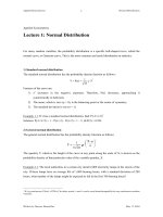
The normal distribution has the following properties:
1. It is bell-shaped.
2. The mean, median, and mode are at the center of the distribution.
3. It is symmetric about the mean. (This means that it is a reflection of
itself if a mean was placed at the center.)
4. It is continuous; i.e., there are no gaps.
5. It never touches the x axis.
6. The total area under the curve is 1 or 100%.
7. About 0.68 or 68% of the area under the curve falls within one
standard deviation on either side of the mean. (Recall that " is the
symbol for the mean and ' is the symbol for the standard deviation.)
About 0.95 or 95% of the area under the curve falls within two
standard deviations of the mean.
About 1.00 or 100% of the area falls within three standard deviations
of the mean. (Note: It is somewhat less than 100%, but for simplicity,
100% will be used here.) See Figure 9-1.
CHAPTER 9 The Normal Distribution
156
EXAMPLE: The mean commuting time between a person’s home and office
is 24 minutes. The standard deviation is 2 minutes. Assume the variable is
normally distributed. Find the probability that it takes a person between

24 and 28 minutes to get to work.
SOLUTION:
Draw the normal distribution and place the mean, 24, at the center. Then
place the mean plus one standard deviation (26) to the right, the mean plus
two standard deviations (28) to the right, the mean plus three standard
deviations (30) to the right, the mean minus one standard deviation (22) to
the left, the mean minus two standard deviations (20) to the left, and the
mean minus three standard deviations (18) to the left, as shown in Figure 9-2.
Using the areas shown in Figure 9-1, the area under the curve between 24
and 28 minutes is 0.341 þ 0.136 ¼ 0.477 or 47.7%. Hence the probability that
the commuter will take between 24 and 28 minutes is about 48%.
Fig. 9-1.
Fig. 9-2.
CHAPTER 9 The Normal Distribution
157
EXAMPLE: According to a study by A.C. Neilson, children between 2 and 5
years of age watch an average of 25 hours of television per week. Assume the
variable is approximately normally distributed with a standard deviation
of 2. If a child is selected at random, find the probability that the child
watched more than 27 hours of television per week.
SOLUTION:
Draw the normal distribution curve and place 25 at the center; then place
27, 29, and 31 to the right corresponding to one, two, and three standard
deviations above the mean, and 23, 21, and 19 to the left corresponding to
one, two, and three standard deviations below the mean. Now place the
areas (percents) on the graph. See Figure 9-3.
Since we are finding the probabilities for the number of hours greater than
27, add the areas of 0.136 þ 0.023 ¼ 0.159 or 15.9%. Hence, the probability is
about 16%.
EXAMPLE: The scores on a national achievement exam are normally

distributed with a mean of 500 and a standard deviation of 100. If a student
who took the exam is randomly selected, find the probability that the student
scored below 600.
SOLUTION:
Draw the normal distribution curve and place 500 at the center. Place
600, 700, and 800 to the right and 400, 300, and 200 to the left, corresponding
to one, two, and three standard deviations above and below the mean respec-
tively. Fill in the corresponding areas. See Figure 9-4.
Fig. 9-3.
CHAPTER 9 The Normal Distribution
158