Thuật toán Algorithms (Phần 38)

CLOSEST POINT PROBLEMS 363

l
L
J
M
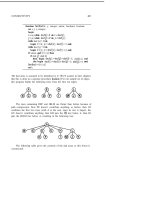
A vertical dividing line just to the right of F has eight points to the left, eight
points to the right. The closest pair on the left half is AC (or AO), the closest
pair on the right is JM. If we have the points sorted on then the closest pair
which is split by the line is found by checking the pairs HI, CI, FK, which is
the closest pair in the whole point set, and finally EK.
Though this algorithm is simply stated, some care is required to imple-
ment it efficiently: for example, it would be too expensive to sort the points
on y within our recursive subroutine. We’ve seen several algorithms with a
running time described by the recurrence T(N) = which implies
that T(N) is proportional to log if we were to do the full sort on y, then
the recurrence would become T(N) = Nlog and it turns out
that this implies that is proportional to N. To avoid this, we
need to avoid the sort of y.
The solution to this problem is simple, but subtle. The mergesort method
from Chapter 12 is based on dividing the elements to be sorted exactly as
the points are divided above. We have two problems to solve and the same
general method to solve them, so we may as well solve them simultaneously!
Specifically, we’ll write one recursive routine that both sorts on y and finds the
closest pair. It will do so by splitting the point set in half, then calling itself
recursively to sort the two halves on y and find the closest pair in each half,
364
CHAPTER 28
then merging to complete the sort on y and applying the procedure above to
complete the closest pair computation. In this way, we avoid the cost of doing
an extra y sort by intermixing the data movement required for the sort with

the data movement required for the closest pair computation.
For the y sort, the split in half could be done in any way, but for
the closest pair computation, it’s required that the points in one half all
have smaller coordinates than the points in the other half. This is easily
accomplished by sorting on x before doing the division. In fact, we may as
well use the same routine to sort on Once this general plan is accepted,
the implementation is not difficult to understand.
As mentioned above, the implementation will use the recursive sort and
merge procedures of Chapter 12. The first step is to modify the list structures
to hold points instead of keys, and to modify merge to check a global variable
pass to decide how to do its comparison. If the comparison should
be done using the x coordinates of the two points; if pass=2 we do the y
coordinates of the two points. The dummy node which appears at the
end of all lists will contain a “sentinel” point with artificially high and y
coordinates.
The next step is to modify the recursive sort of Chapter 12 also to do the
closest-point computation when This is done by replacing the line
containing the call to merge and the recursive calls to sort in that program
by the following code:
if pass=2 then
div div 2)));
if pass=2 then
begin

repeat
if then
begin

end
until a=z
end
CLOSEST POINT PROBLEMS
365
If this is straight mergesort: it returns a linked list containing the
points sorted on their coordinates (because of the change to merge). The
magic of this implementation comes when The program not only sorts
on y but also completes the closest-point computation, as described in detail
below. The procedure check simply checks whether the distance between the
two points given as arguments is less than the global variable min. If so, it
resets min to that distance and saves the points in the global variables cpl
and Thus, the global min always contains the distance between cpl and
the closest pair found so far.
First, we sort on x, then we sort on y and find the closest pair by invoking
sort as follows:
new(z);

new(h);
N);
N);
After these calls, the closest pair of points is found in the global variables
and which are managed by the check “find the minimum” procedure.
The crux of the implementation is the operation of sort when
Before the recursive calls the points are sorted on x: this ordering is used to
divide the points in half and to find the x coordinate of the dividing line.
the recursive calls the points are sorted on y and the distance between every
pair of points in each half is known to be greater than min. The ordering on

y is used to scan the points near the dividing line; the value of min is used to
limit the number of points to be tested. Each point within a distance of min
of the dividing line is checked against each of the previous four points found
within a distance of min of the dividing line. This is guaranteed to find any
pair of points closer together than min with one member of the pair on either
side of the dividing line. This is an amusing geometric fact which the reader
may wish to check. (We know that points which fall on the same side of the
dividing line are spaced by at least min, so the number of points falling in any
circle of radius min is limited.)
It is interesting to examine the order in which the various vertical dividing
lines are tried in this algorithm. This can be described with the aid of the
following binary tree:
CHAPTER 28
G OA DE CH KB PN JM L
Each node in this tree represents a vertical line dividing the points in the left
and right The nodes are numbered in the order in which the vertical
lines are tried in the algorithm. Thus, first the line between G and 0 is tried
and the pair GO is retained as the closest so far. Then the line between A and
D is tried, but A and D are too far apart to change min. Then the line between
0 and A is tried and the pairs GD and OA all are successively closer pairs.
It happens for this example that no closer pairs are found until FK, which is
the last pair checked for the last dividing line tried. This diagram reflects the
difference between top-down and bottom-up mergesort. A bottom-up version
of the closest-pair problem can be developed in the same way as for mergesort,
which would be described by a tree like the one above, numbered left to right
and bottom to top.
The general approach that we’ve used for the closest-pair problem can
be used to solve other geometric problems. For example, another problem of
interest is the all-nearest-neighbors problem: for each point we want to find
the point nearest to it. This problem can be solved using a program like the

one above with extra processing along the dividing line to find, for each point,
whether there is a point on the other side closer than its closest point on its
own side. Again, the “free” y sort is helpful for this computation.
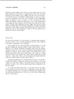
Voronoi Diagrams
The set of all points closer to a given point in a point set than to all other points
in the set is an interesting geometric structure called the Voronoi polygon for
the point. The union of all the Voronoi polygons for a point set is called its
Voronoi diagram. This is the ultimate in closest-point computations: we’ll see
that most of the problems involving distances between points that we face
have natural and interesting solutions based on the Voronoi diagram. The
diagram for our sample point set is comprised of the thick lines in the diagram
below:
CLOSEST POINT PROBLEMS 367
Basically, the Voronoi polygon for a point is made up of the perpendicular
bisectors separating the point from those points closest to it. The actual
definition is the other way around: the Voronoi polygon is defined to be the
set of all points in the plane closer to the given point than to any other point
in the point set, and the points “closest to” a point are defined to be those that
lead to edges on the Voronoi polygon. The dual of the Voronoi diagram makes
this correspondence explicit: in the dual, a line is drawn between each point
and all the points “closest to” it. Put another way, x and y are connected in
the Voronoi dual if their Voronoi polygons have an edge in common. The dual
for our example is comprised of the thin dotted lines in the above diagram.
The Voronoi diagram and its dual have many properties that lead to
efficient algorithms for closest-point problems. The property that makes these
algorithms efficient is the number of lines in both the diagram and the
dual is proportional to a small constant times For example, the line
connecting the closest pair of points must be in the dual, so the problem of
the previous section can be solved by computing the dual and then simply
finding the minimum length line among the lines in the dual. Similarly, the

line connecting each point to its nearest neighbor must be in the dual, so the
all-nearest-neighbors problem reduces directly to finding the dual. The convex
hull of the point set is part of the dual, so computing the Voronoi dual is yet