Thuật toán Algorithms (Phần 39)

29. Elementary Graph Algorithms
A great many problems are naturally formulated in terms of objects
and connections between them. For example, given an airline route
map of the eastern U. S., we might be interested in questions like: “What’s
the fastest way to get from Providence to Princeton?” Or we might be more
interested in money than in time, and look for the cheapest way to get from
Providence to Princeton. To answer such questions we need only information
about interconnections (airline routes) between objects (towns).
Electric circuits are another obvious example where interconnections be-
tween objects play a central role. Circuit elements like transistors, resistors,
and capacitors are intricately wired together. Such circuits can be represented
and processed within a computer in order to answer simple questions like “Is
everything connected together?” as well as complicated questions like “If
this circuit is built, will it work?” In this case, the answer to the first ques-
tion depends only on the properties of the interconnections (wires), while the
answer to the second question requires detailed information about both the
wires and the objects that they connect.
A third example is “job scheduling,” where the objects are tasks to be
performed, say in a manufacturing process, and interconnections indicate
which jobs should be done before others. Here we might be interested in
answering questions like “When should each task be performed?”
A graph is a mathematical object which accurately models such situations.
In this chapter, we’ll examine some basic properties of graphs, and in the next
several chapters we’ll study a variety of algorithms for answering questions of
the type posed above.
Actually, we’ve already encountered graphs in several instances in pre-
vious chapters. Linked data structures are actually representations of graphs,
and some of the algorithms that we’ll see for processing graphs are similar to
algorithms that we’ve already seen for processing trees and other structures.
373
374

CHAPTER 29
For example, the finite-state machines of Chapters 19 and 20 are represented
with graph structures.
Graph theory is a major branch of combinatorial mathematics and has
been intensively studied for hundreds of years. Many important and useful
properties of graphs have been proved, but many difficult problems have yet to
be resolved. We’ll be able here only to scratch the surface of what is known
about graphs, covering enough to be able to understand the fundamental
algorithms.
As with so many of the problem domains that we’ve studied, graphs
have only recently begun to be examined from an algorithmic point of view.
Although some of the fundamental algorithms are quite old, many of the
interesting ones have been discovered within the last ten years. Even trivial
graph algorithms lead to interesting computer programs, and the nontrivial
algorithms that we’ll examine are among the most elegant and interesting
(though difficult to understand) algorithms known.
Glossary
A good deal of nomenclature is associated with graphs. Most of the terms
have straightforward definitions, and it is convenient to put them in one place
even though we won’t be using some of them until later.
A graph is a collection of vertices and edges. Vertices are simple objects
which can have names and other properties; an edge is connection between
two vertices. One can draw a graph by marking points for the vertices and
drawing lines connecting them for the edges, but it must be borne in mind
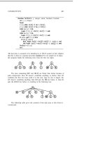
that the graph is defined independently of the representation. For example,
the following two drawings represent the same graph:
We define this graph by saying that it consists of the set of vertices A B C D
E F G H I J K L M and the set of edges between these vertices AG Al3 AC
LMJMJLJKEDFDHIFEAF’GE.
ELEMENTARY ALGORITHMS

375
For some applications, such as the airline route example above, it might
not make sense to rearrange the placement of the vertices as in the diagrams
above. But for some other applications, such as the electric circuit application
above, it is best to concentrate only on the edges and vertices, independent
of any particular geometric placement. And for still other applications, such
as the finite-state machines in Chapters 19 and 20, no particular geometric
placement of nodes is ever implied. The relationship between graph algorithms
and geometric problems is discussed in further detail in Chapter 31. For now,
we’ll concentrate on “pure” graph algorithms which process simple collections
of edges and nodes.
A path from vertex x to y in a graph is a list of vertices in which successive
vertices are connected by edges in the graph. For example, BAFEG is a path
from B to G in the graph above. A graph is connected if there is a path
from every node to every other node in the graph. Intuitively, if the vertices
were physical objects and the edges were strings connecting them, a connected
graph would stay in one piece if picked up by any vertex. A graph which is
not connected is made up of connected components; for example, the graph
drawn above has three connected components. A simple path is a path in
which no vertex is repeated. (For example, BAFEGAC is not a simple path.)
A cycle is a path which is simple except that the first and last vertex are the
same (a path from a point back to itself): the path AFEGA is a cycle.
A graph with no cycles is called a tree. There is only one path between
any two nodes in a tree. (Note that binary trees and other types of trees that
we’ve built with algorithms are special cases included in this general definition
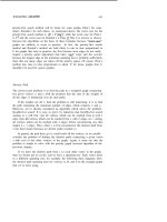
of trees.) A group of disconnected trees is called a forest. A spanning tree of a
graph is a that contains all the vertices but only enough of the edges
to form a tree. For example, below is a spanning tree for the large component
of our sample graph.
Note that if we add any edge to a tree, it must form a cycle (because

there is already a path between the two vertices that it connects). Also, it is
easy to prove by induction that a tree on V vertices has exactly V 1 edges.
376
CHAPTER 29
If a graph with V vertices has less than V 1 edges, it can’t be connected.
If it has more that V 1 edges, it must have a cycle. (But if it has exactly
V 1 edges, it need not be a tree.)
We’ll denote the number of vertices in a given graph by V, the number
of edges by E. Note that E can range anywhere from 0 to 1). Graphs
with all edges present are called complete graphs; graphs with relatively few
edges (say less than Vlog V) are called sparse; graphs with relatively few of
the possible edges missing are called dense.
This fundamental dependence on two parameters makes the comparative
study of graph algorithms somewhat more complicated than many algorithms
that we’ve studied, because more possibilities arise. For example, one algo-
rithm might take about steps, while another algorithm for the same prob-
lem might take (E V) log E steps. The second algorithm would be better for
sparse graphs, but the first would be preferred for dense graphs.
Graphs as defined to this point are called undirected graphs, the simplest
type of graph. We’ll also be considering more complicated type of graphs, in
which more information is associated with the nodes and edges. In weighted
graphs integers (weights) are assigned to each edge to represent, say, distances
or costs. In directed graphs , edges are “one-way”: an edge may go from x to
y but not the other way. Directed weighted graphs are sometimes called net-
works. As we’ll discover, the extra information weighted and directed graphs
contain makes them somewhat more difficult to manipulate than simple un-
directed graphs.
Representation
In order to process graphs with a computer program, we first need to decide
how to represent them within the computer. We’ll look at two commonly used

representations; the choice between them depends whether the graph is dense
or sparse.
The first step in representing a graph is to map the vertex names to
integers between 1 and V. The main reason for doing this is to make it
possible to quickly access information corresponding to each vertex, using
array indexing. Any standard searching scheme can be used for this purpose:
for instance, we can translate vertex names to integers between 1 and V
by maintaining a hash table or a binary tree which can be searched to
the integer corresponding to any given vertex name. Since we have already
studied these techniques, we’ll assume that we have available a function index
to convert from vertex names to integers between 1 and V and a function name
to convert from integers to vertex names. In order to make the algorithms easy
to follow, our examples will use one-letter vertex names, with the ith letter
of the alphabet corresponding to the integer i. Thus, though name and index
ELEMENTARY GRAPH ALGORITHMS 377
are trivial to implement for our examples, their use makes it easy to extend
the algorithms to handle graphs with real vertex names using techniques from
Chapters 14-17.
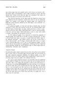
The most straightforward representation for graphs is the so-called
jacenc y matrix representation. A V-by-V array of boolean values is main-
tained, with set to true if there is an edge from vertex x to vertex y
and false otherwise. The adjacency matrix for our example graph is given
below.
ABCDEFGHIJKLM
A1110011000000
10000000110000
KOOOOOOOOO1 1 0 0
Notice that each edge is really represented by two bits: an edge connecting
x and y is represented by true values in both and x]. While it
is possible to save space by storing only half of this symmetric matrix, it

is inconvenient to do so in Pascal and the algorithms are somewhat simpler
with the full matrix. Also, it’s sometimes convenient to assume that there’s
an “edge” from each vertex to itself, so x] is set to 1 for x from 1 to V.
A graph is defined by a set of nodes and a set of edges connecting them.
To read in a graph, we need to settle on a format for reading in these sets.
The obvious format to use is first to read in the vertex names and then read
in pairs of vertex names (which define edges). As mentioned above, one easy
way to proceed is to read the vertex names into a hash table or binary search
tree and to assign to each vertex name an integer for use in accessing
indexed arrays like the adjacency matrix. The ith vertex read can be assigned
the integer (Also, as mentioned above, we’ll assume for simplicity in our
examples that the vertices are the first V letters of the alphabet, so that we
can read in graphs by reading V and E, then E pairs of letters from the first