Xử lý hình ảnh thông minh P6

Intelligent Image Processing.SteveMann
Copyright  2002 John Wiley & Sons, Inc.
ISBNs: 0-471-40637-6 (Hardback); 0-471-22163-5 (Electronic)
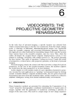
6
VIDEOORBITS: THE
PROJECTIVE GEOMETRY
RENAISSANCE
In the early days of personal imaging, a specific location was selected from
which a measurement space or the like was constructed. From this single vantage
point, a collection of differently illuminated/exposed images was constructed
using the wearable computer and associated illumination apparatus. However,
this approach was often facilitated by transmitting images from a specific location
(base station) back to the wearable computer, and vice versa. Thus, when the
author developed the eyeglass-based computer display/camera system, it was
natural to exchange viewpoints with another person (i.e., the person operating
the base station). This mode of operation (“seeing eye-to-eye”) made the notion
of perspective a critical factor, with projective geometry at the heart of personal
imaging.
Personal imaging situates the camera such that it provides a unique first-person
perspective. In the case of the eyeglass-mounted camera, the machine captures
the world from the same perspective as its host (human).
In this chapter we will consider results of a new algorithm of projective geom-
etry invented for such applications as “painting” environmental maps by looking
around, wearable tetherless computer-mediated reality, the new genre of personal
documentary that arises from this mediated reality, and the creation of a collective
adiabatic intelligence arising from shared mediated-reality environments.
6.1 VIDEOORBITS
Direct featureless methods are presented for estimating the 8 parameters of an
“exact” projective (homographic) coordinate transformation to register pairs of
images, together with the application of seamlessly combining a plurality of
images of the same scene. The result is a single image (or new image sequence)

233
234
VIDEOORBITS: THE PROJECTIVE GEOMETRY RENAISSANCE
of greater resolution or spatial extent. The approach is “exact” for two cases of
static scenes: (1) images taken from the same location of an arbitrary 3-D scene,
with a camera that is free to pan, tilt, rotate about its optical axis, and zoom
and (2) images of a flat scene taken from arbitrary locations. The featureless
projective approach generalizes interframe camera motion estimation methods
that have previously used an affine model (which lacks the degrees of freedom to
“exactly” characterize such phenomena as camera pan and tilt) and/or that have
relied upon finding points of correspondence between the image frames. The
featureless projective approach, which operates directly on the image pixels, is
shown to be superior in accuracy and ability to enhance resolution. The proposed
methods work well on image data collected from both good-quality and poor-
quality video under a wide variety of conditions (sunny, cloudy, day, night).
These new fully automatic methods are also shown to be robust to deviations
from the assumptions of static scene and to exhibit no parallax.
Many problems require finding the coordinate transformation between two
images of the same scene or object. In order to recover camera motion between
video frames, to stabilize video images, to relate or recognize photographs taken
from two different cameras, to compute depth within a 3-D scene, or for image
registration and resolution enhancement, it is important to have a precise descrip-
tion of the coordinate transformation between a pair of images or video frames
and some indication as to its accuracy.
Traditional block matching (as used in motion estimation) is really a special
case of a more general coordinate transformation. In this chapter a new solution to
the motion estimation problem is demonstrated, using a more general estimation
of a coordinate transformation, and techniques for automatically finding the 8-
parameter projective coordinate transformation that relates two frames taken of
the same static scene are proposed. It is shown, both by theory and example,

how the new approach is more accurate and robust than previous approaches
that relied upon affine coordinate transformations, approximations to projective
coordinate transformations, and/or the finding of point correspondences between
the images. The new techniques take as input two frames, and automatically
output the 8 parameters of the “exact” model, to properly register the frames.
They do not require the tracking or correspondence of explicit features, yet they
are computationally easy to implement.
Although the theory presented makes the typical assumptions of static scene
and no parallax, It is shown that the new estimation techniques are robust to
deviations from these assumptions. In particular, a direct featureless projective
parameter estimation approach to image resolution enhancement and compositing
is applied, and its success on a variety of practical and difficult cases, including
some that violate the nonparallax and static scene assumptions, is illustrated.
An example image composite, made with featureless projective parameter esti-
mation, is reproduced in Figure 6.1 where the spatial extent of the image is
increased by panning the camera while compositing (e.g., by making a panorama),
and the spatial resolution is increased by zooming the camera and by combining
overlapping frames from different viewpoints.
BACKGROUND
235
Figure 6.1 Image composite made from three image regions (author moving between two
different locations) in a large room: one image taken looking straight ahead (outlined in a
solid line); one image taken panning to the left (outlined in a dashed line); one image taken
panning to the right with substantial zoom-in (outlined in a dot-dash line). The second two
have undergone a coordinate transformation to put them into the same coordinates as the
first outlined in a solid line (the reference frame). This composite, made from NTSC-resolution
images, occupies about 2000 pixels across and shows good detail down to the pixel level.
Note the increased sharpness in regions visited by the zooming-in, compared to other areas.
(See magnified portions of composite at the sides.) This composite only shows the result of
combining three images, but in the final production, many more images can be used, resulting

in a high-resolution full-color composite showing most of the large room. (Figure reproduced
from [63], courtesy of IS&T.)
6.2 BACKGROUND
Hundreds of papers have been published on the problems of motion estimation
and frame alignment (for review and comparison, see [94]). In this section the
basic differences between coordinate transformations is reviewed and the impor-
tance of using the “exact” 8-parameter projective coordinate transformation is
emphasized.
6.2.1 Coordinate Transformations
A coordinate transformation maps the image coordinates, x = [x, y]
T
to a new
set of coordinates, x

= [x

,y

]
T
. The approach to “finding the coordinate trans-
formation” depends on assuming it will take one of the forms in Table 6.1, and
then estimating the parameters (2 to 12 parameters depending on the model) in
the chosen form. An illustration showing the effects possible with each of these
forms is shown in Figure 6.3.
A common assumption (especially in motion estimation for coding, and
optical flow for computer vision) is that the coordinate transformation between
frames is translation. Tekalp, Ozkan, and Sezan [95] have applied this assump-
tion to high-resolution image reconstruction. Although translation is the least
constraining and simplest to implement of the seven coordinate transformations

in Table 6.1, it is poor at handling large changes due to camera zoom, rotation,
pan, and tilt.
Zheng and Chellappa [96] considered the image registration problem using a
subset of the affine model — translation, rotation, and scale. Other researchers
236
VIDEOORBITS: THE PROJECTIVE GEOMETRY RENAISSANCE
Table 6.1 Image Coordinate Transformations
Model Coordinate Transformation from x to x

Parameters
Translation x

= x + bb∈

2
Affine x

= Ax + bA∈

2×2
, b ∈

2
Bilinear x

= q
x

xy
xy + q

x

x
x + q
x

y
y + q
x

y

= q
y

xy
xy + q
y

x
x + q
y

y
y + q
y

q
∗
∈


Projective x

=
Ax + b
c
T
x + 1
A ∈

2×2
, b, c ∈

2
Relative-projective x

=
Ax + b
c
T
x + 1
+ xA∈

2×2
, b, c ∈

2
Pseudoperspective x

= q

x

x
x + q
x

y
y + q
x

+ q
α
x
2
+ q
β
xy
y

= q
y

x
x + q
y

y
y + q
y


+ q
α
xy + q
β
y
2
q
∗
∈

Biquadratic x

= q
x

x
2
x
2
+ q
x

xy
xy + q
x

y
2
y
2

+ q
x

x
x
+ q
x

y
y + q
x

y

= q
y

x
2
x
2
+ q
y

xy
xy + q
y

y
2

y
2
+ q
y

x
x
+ q
y

y
y + q
y

q
∗
∈

(
a
)
(
b
)
(
c
)
(
a,b,c
)

−8 −6 −4 −2 0 2 4 6 8
−8
−6
−4
−2
0
2
4
6
8
Domain coordinate value
Projective"operative function"
Range coordinate value
X
2
X
1
1
c
′
(
d
)
Figure 6.2 The projective chirping phenomenon. (a) A real-world object that exhibits peri-
odicity generates a projection (image) with ‘‘chirping’’ — periodicity in perspective. (b)Center
raster of image. (c) Best-fit projective chirp of form sin[2π((ax + b)/(cx + 1))]. (d) Graphical
depiction of exemplar 1-D projective coordinate transformation of sin(2πx
1
) into a projective
chirp function, sin(2πx

2
) = sin[2π((2x
1
− 2)/(x
1
+ 1))]. The range coordinate as a function of
the domain coordinate forms a rectangular hyperbola with asymptotes shifted to center at
the vanishing point, x
1
=−1/c =−1, and exploding point, x
2
= a/c = 2; the chirpiness is
c

= c
2
/(bc − a) =−
1
4
.
BACKGROUND
237
Nonchirping models
(Original) (Bilinear)(Affine) (Projective)
Chirping models
(Biquadratic)(Pseudo-
perspective)
(Relative-
projective)
Figure 6.3 Pictorial effects of the six coordinate transformations of Table 6.1, arranged left to

right by number of parameters. Note that translation leaves the
ORIGINAL
house figure unchanged,
except in its location. Most important, all but the
AFFINE
coordinate transformation affect the
periodicity of the window spacing (inducing the desired ‘‘chirping,’’ which corresponds to what
we see in the real world). Of these five, only the
PROJECTIVE
coordinate transformation preserves
straight lines. The 8-parameter
PROJECTIVE
coordinate transformation ‘‘exactly’’ describes the
possible image motions (‘‘exact’’ meaning under the idealized zero-parallax conditions).
[72,97] have assumed affine motion (six parameters) between frames. For the
assumptions of static scene and no parallax, the affine model exactly describes
rotation about the optical axis of the camera, zoom of the camera, and pure
shear, which the camera does not do, except in the limit as the lens focal length
approaches infinity. The affine model cannot capture camera pan and tilt, and
therefore cannot properly express the “keystoning” (projections of a rectangular
shape to a wedge shape) and “chirping” we see in the real world. (By “chirping”
what is meant is the effect of increasing or decreasing spatial frequency with
respect to spatial location, as illustrated in Fig. 6.2) Consequently the affine
model attempts to fit the wrong parameters to these effects. Although it has
fewer parameters, the affine model is more susceptible to noise because it lacks
the correct degrees of freedom needed to properly track the actual image motion.
The 8-parameter projective model gives the desired 8 parameters that exactly
account for all possible zero-parallax camera motions; hence there is an important
need for a featureless estimator of these parameters. The only algorithms proposed
to date for such an estimator are [63] and, shortly after, [98]. In both algorithms

a computationally expensive nonlinear optimization method was presented. In the
earlier publication [63] a direct method was also proposed. This direct method
uses simple linear algebra, and it is noniterative insofar as methods such as
238
VIDEOORBITS: THE PROJECTIVE GEOMETRY RENAISSANCE
Levenberg–Marquardt, and the like, are in no way required. The proposed method
instead uses repetition with the correct law of composition on the projective
group, going from one pyramid level to the next by application of the group’s
law of composition. The term “repetitive” rather than “iterative” is used, in partic-
ular, when it is desired to distinguish the proposed method from less preferable
iterative methods, in the sense that the proposed method is direct at each stage of
computation. In other words, the proposed method does not require a nonlinear
optimization package at each stage.
Because the parameters of the projective coordinate transformation had tradi-
tionally been thought to be mathematically and computationally too difficult to
solve, most researchers have used the simpler affine model or other approxima-
tions to the projective model. Before the featureless estimation of the parameters
of the “exact” projective model is proposed and demonstrated, it is helpful to
discuss some approximate models.
Going from first order (affine), to second order, gives the 12-parameter
biquadratic model. This model properly captures both the chirping (change
in spatial frequency with position) and converging lines (keystoning) effects
associated with projective coordinate transformations. It does not constrain
chirping and converging to work together (the example in Fig. 6.3 being chosen
with zero convergence yet substantial chirping, illustrates this point). Despite
its larger number of parameters, there is still considerable discrepancy between
a projective coordinate transformation and the best-fit biquadratic coordinate
transformation. Why stop at second order? Why not use a 20-parameter bicubic
model? While an increase in the number of model parameters will result in a
better fit, there is a trade-off where the model begins to fit noise. The physical

camera model fits exactly in the 8-parameter projective group; therefore we know
that eight are sufficient. Hence it seems reasonable to have a preference for
approximate models with exactly eight parameters.
The 8-parameter bilinear model seems to be the most widely used model [99]
in image processing, medical imaging, remote sensing, and computer graphics.
This model is easily obtained from the biquadratic model by removing the four
x
2
and y
2
terms. Although the resulting bilinear model captures the effect of
converging lines, it completely fails to capture the effect of chirping.
The 8-parameter pseudoperspective model [100] and an 8-parameter relative-
projective model both capture the converging lines and the chirping of a
projective coordinate transformation. The pseudoperspective model, for example,
may be thought of as first a means of removal of two of the quadratic terms
(q
x

y
2
= q
y

x
2
= 0), which results in a 10- parameter model (the q-chirp of [101])
and then of constraining the four remaining quadratic parameters to have two
degrees of freedom. These constraints force the chirping effect (captured by
q

x

x
2
and q
y

y
2
) and the converging effect (captured by q
x

xy
and q
y

xy
)towork
together to match as closely as possible the effect of a projective coordinate
transformation. In setting q
α
= q
x

x
2
= q
y

xy

, the chirping in the x-direction is
forced to correspond with the converging of parallel lines in the x-direction (and
likewise for the y-direction).
BACKGROUND
239
Of course, the desired “exact” 8 parameters come from the projective model,
but they have been perceived as being notoriously difficult to estimate. The
parameters for this model have been solved by Tsai and Huang [102], but their
solution assumed that features had been identified in the two frames, along
with their correspondences. The main contribution of this chapter is a simple
featureless means of automatically solving for these 8 parameters.
Other researchers have looked at projective estimation in the context of
obtaining 3-D models. Faugeras and Lustman [83], Shashua and Navab [103],
and Sawhney [104] have considered the problem of estimating the projective
parameters while computing the motion of a rigid planar patch, as part of a larger
problem of finding 3-D motion and structure using parallax relative to an arbitrary
plane in the scene. Kumar et al. [105] have also suggested registering frames of
video by computing the flow along the epipolar lines, for which there is also
an initial step of calculating the gross camera movement assuming no parallax.
However, these methods have relied on feature correspondences and were aimed
at 3-D scene modeling. My focus is not on recovering the 3-D scene model,
but on aligning 2-D images of 3-D scenes. Feature correspondences greatly
simplify the problem; however, they also have many problems. The focus of this
chapter is simple featureless approaches to estimating the projective coordinate
transformation between image pairs.
6.2.2 Camera Motion: Common Assumptions and Terminology
Two assumptions are typically made in this area of research. The first is that
the scene is constant — changes of scene content and lighting are small between
frames. The second is that of an ideal pinhole camera — implying unlimited
depth of field with everything in focus (infinite resolution) and implying that

straight lines map to straight lines.
1
Consequently the camera has three degrees
of freedom in 2-D space and eight degrees of freedom in 3-D space: translation
(X, Y , Z), zoom (scale in each of the image coordinates x and y), and rotation
(rotation about the optical axis), pan, and tilt. These two assumptions are also
made in this chapter.
In this chapter an “uncalibrated camera” refers to one in which the principal
point
2
is not necessarily at the center (origin) of the image and the scale is not
necessarily isotropic
3
It is assumed that the zoom is continually adjusted by the
camera user, and that we do not know the zoom setting, or whether it was changed
between recording frames of the image sequence. It is also assumed that each
element in the camera sensor array returns a quantity that is linearly proportional
1
When using low-cost wide-angle lenses, there is usually some barrel distortion, which we correct
using the method of [106].
2
The principal point is where the optical axis intersects the film.
3
Isotropic means that magnification in the x and y directions is the same. Our assumption facilitates
aligning frames taken from different cameras.
240
VIDEOORBITS: THE PROJECTIVE GEOMETRY RENAISSANCE
Table 6.2 Two No Parallax Cases for a Static Scene
Scene Assumptions Camera Assumptions
Case 1 Arbitrary 3-D Free to zoom, rotate, pan, and tilt, fixed COP

Case 2 Planar Free to zoom, rotate, pan, and tilt, free to translate
Note: The first situation has 7 degrees of freedom (yaw, pitch, roll, translation in each of the
3 spatial axes, and zoom), while the second has 4 degrees of freedom (pan, tilt, rotate, and
zoom). Both, however, are represented within the 8 scalar parameters of the projective group
of coordinate transformations.
to the quantity of light received.
4
With these assumptions, the exact camera
motion that can be recovered is summarized in Table 6.2.
6.2.3 Orbits
Tsai and Huang [102] pointed out that the elements of the projective group give
the true camera motions with respect to a planar surface. They explored the
group structure associated with images of a 3-D rigid planar patch, as well as the
associated Lie algebra, although they assume that the correspondence problem
has been solved. The solution presented in this chapter (which does not require
prior solution of correspondence) also depends on projective group theory. The
basics of this theory are reviewed, before presenting the new solution in the next
section.
Projective Group in 1-D Coordinates
A group is a set upon which there is defined an associative law of composition
(closure, associativity), which contains at least one element (identity) whose
composition with another element leaves it unchanged, and for which every
element of the set has an inverse.
A group of operators together with a set of operands form a group operation.
5
In this chapter coordinate transformations are the operators (group) and images
are the operands (set). When the coordinate transformations form a group, then
two such coordinate transformations, p
1
and p

2
, acting in succession, on an image
(e.g., p
1
acting on the image by doing a coordinate transformation, followed by
a further coordinate transformation corresponding to p
2
, acting on that result)
can be replaced by a single coordinate transformation. That single coordinate
transformation is given by the law of composition in the group.
The orbit of a particular element of the set, under the group operation [107],
is the new set formed by applying to it all possible operators from the group.
4
This condition can be enforced over a wide range of light intensity levels, by using the Wyckoff
principle [75,59].
5
Also known as a group action or G-set [107].
BACKGROUND
241
6.2.4 VideoOrbits
Here the orbit of particular interest is the collection of pictures arising from one
picture through applying all possible projective coordinate transformations to that
picture. This set is referred to as the VideoOrbit of the picture in question. Image
sequences generated by zero-parallax camera motion on a static scene contain
images that all lie in the same VideoOrbit.
The VideoOrbit of a given frame of a video sequence is defined to be the
set of all images that can be produced by applying operators from the projective
group to the given image. Hence the coordinate transformation problem may be
restated: Given a set of images that lie in the same orbit of the group, it is desired
to find for each image pair, that operator in the group which takes one image to

the other image.
If two frames, f
1
and f
2
, are in the same orbit, then there is an group operation,
p, such that the mean-squared error (MSE) between f
1
and f

2
= p ◦ f
2
is zero.
In practice, however, the goal is to find which element of the group takes one
image “nearest” the other, for there will be a certain amount of parallax, noise,
interpolation error, edge effects, changes in lighting, depth of focus, and so on.
Figure 6.4 illustrates the operator p acting on frame f
2
to move it nearest to frame
f
1
. (This figure does not, however, reveal the precise shape of the orbit, which
occupies a 3-D parameter space for 1-D images or an 8-D parameter space for 2-
D images.) For simplicity the theory is reviewed first for the projective coordinate
transformation in one dimension.
6
Suppose that we take two pictures, using the same exposure, of the same
scene from fixed common location (e.g., where the camera is free to pan, tilt,
and zoom between taking the two pictures). Both of the two pictures capture the

(
a
)(
b
)
1
2
1
2
Figure 6.4 Video orbits. (a) The orbit of frame 1 is the set of all images that can be produced
by acting on frame 1 with any element of the operator group. Assuming that frames 1 and 2
are from the same scene, frame 2 will be close to one of the possible projective coordinate
transformations of frame 1. In other words, frame 2 ‘‘lies near the orbit of’’ frame 1. (b)By
bringing frame 2 along its orbit, we can determine how closely the two orbits come together at
frame 1.
6
In this 2-D world, the “camera” consists of a center of projection (pinhole “lens”) and a line (1-D
sensor array or 1-D “film”).
242
VIDEOORBITS: THE PROJECTIVE GEOMETRY RENAISSANCE
same pencil of light,
7
but each projects this information differently onto the film
or image sensor. Neglecting that which falls beyond the borders of the pictures,
each picture captures the same information about the scene but records it in a
different way. The same object might, for example, appear larger in one image
than in the other, or might appear more squashed at the left and stretched at
the right than in the other. Thus we would expect to be able to construct one
image from the other, so that only one picture should need to be taken (assuming
that its field of view covers all the objects of interest) in order to synthesize

all the others. We first explore this idea in a make-believe “Flatland” where
objects exist on the 2-D page, rather than the 3-D world in which we live, and
where pictures are real-valued functions of one real variable, rather than the more
familiar real-valued functions of two real-variables.
For the two pictures of the same pencil of light in Flatland, a common COP is
defined at the origin of our coordinate system in the plane. In Figure 6.5 a single
camera that takes two pictures in succession is depicted as two cameras shown
together in the same figure. Let Z
k
, k ∈{1, 2} represent the distances, along
each optical axis, to an arbitrary point in the scene, P ,andletX
k
represent the
distances from P to each of the optical axes. The principal distances are denoted
z
k
. In the example of Figure 6.5, we are zooming in (increased magnification) as
we go from frame 1 to frame 2.
Considering an arbitrary point P in the scene, subtending in a first picture
an angle α = arctan(x
1
/z
1
) = arctan(x
1
/z
1
), the geometry of Figure 6.5 defines
a mapping from x
1

to x
2
, based on a camera rotating through an angle of θ
between the taking of two pictures [108,17]:
x
2
= z
2
tan(arctan

x
1
z
1

− θ) ∀x
1
= o
1
,(6.1)
where o
1
= z
1
tan(π/2 + θ) is the location of the singularity in the domain x
1
.
This singularity is known as the “appearing point” [17]. The mapping (6.1)
defines the coordinate transformation between any two pictures of the same
subject matter, where the camera is free to pan, and zoom, between the taking of

these two pictures. Noise (movement of subject matter, change in illumination,
or circuit noise) is neglected in this simple model. There are three degrees of
freedom, namely the relative angle θ, through which the camera rotated between
taking of the two pictures, and the zoom settings, z
1
and z
2
.
Unfortunately, this mapping (6.1) involves the evaluation of trigonometric
functions at every point x
1
in the image domain. However, (6.1) can be rearranged
in a form that only involves trigonometric calculations once per image pair, for
the constants defining the relation between a particular pair of images.
7
We neglect the boundaries (edges or ends of the sensor) and assume that both pictures have sufficient
field of view to capture all of the objects of interest.
BACKGROUND
243
Z
2
Z
1
z
1
X
1
X
2
z

2
COP
x
1
p
1
x
2
p
2
Scene
q
a
P
Figure 6.5 Camera at a fixed location. An arbitrary scene is photographed twice, each time
with a different camera orientation and a different principal distance (zoom setting). In both
cases the camera is located at the same place (COP) and thus captures the same pencil of
light. The dotted line denotes a ray of light traveling from an arbitrary point P in the scene to the
COP. Heavy lines denote both camera optical axes in each of the two orientations as well as
the image sensor in each of its two pan and zoom positions. The two image sensors (or films)
are in front of the camera to simplify mathematical derivations.
First, note the well-known trigonometric identity for the difference of two
angles:
tan(α − θ) =
tan(α) − tan(θ)
1 + tan(α) tan(θ)
.(6.2)
Substitute into the equation tan(α) = x
1
/z

1
. Thus
x
2
= z
2
x
1
/z
1
− tan(θ)
1 + (x
1
/z
1
) tan(θ )
(6.3)
Letting constants a = z
2
/z
1
, b =−z
2
tan(θ),andc = tan(θ)/z
1
, the trigono-
metric computations are removed from the independent variable, so that
x
2
=

ax
1
+ b
cx
1
+ 1
∀x
1
= o
1
,(6.4)
244
VIDEOORBITS: THE PROJECTIVE GEOMETRY RENAISSANCE
where o
1
= z
1
tan(π/2 + θ) =−1/c, is the location of the singularity in the
domain.
It should be emphasized that if we set c = 0, we arrive at the affine group,
upon which the popular wavelet transform is based. Recall that c, the degree of
perspective, has been given the interpretation of a chirp rate [108] and forms the
basis for the p-chirplet transform.
Let p ∈ P denote a particular mapping from x
1
to x
2
, governed by the
three parameters (three degrees of freedom) of this mapping, p


= [z
1
,z
2
,θ],
or equivalently by a, b,andc from (6.4).
Now, within the context of the VideoOrbits theory [2], it is desired that the
set of coordinate transformations set forth in (6.4) form a group of coordinate
transformations. Thus it is desired that:
•
any two coordinate transformations of this form, when composed, form
another coordinate transformation also of this form, which is the law of
composition;
•
the law of composition be associative;
•
there exists an identity coordinate transformation;
•
every coordinate transformation in the set has an inverse.
A singular coordinate transformation of the form a = bc does not have an
inverse. However, we do not need to worry about such a singularity because
this situation corresponds to tan
2
(θ) =−1forwhichθ is ComplexInfinity. Thus
such a situation will not happen in practice.
However, a more likely problem is the situation for which θ is 90 degrees,
giving values for b and c that are ComplexInfinity (since tan(π/2) is Complex-
Infinity). This situation can easily happen, if we take a picture, and then swing
the camera through a 90 degree angle and then take another picture, as shown in
Figure 6.6. Thus a picture of a sinusoidally varying surface in the first camera

would appear as a function of the form sin(1/x) in the second camera, and the
coordinate transformation of this special case is given by x
2
= 1/x
1
. More gener-
ally, coordinate transformations of the form x
2
= a
1
/x
1
+ b
1
cannot be expressed
by (6.4).
Accordingly, in order to form a group representation, coordinate transforma-
tions may be expressed as x
2
= (a
1
x
1
+ b
1
)/(c
1
x
1
+ d

1
), ∀a
1
d
1
= b
1
c
1
.Elements
of this group of coordinate transformations are denoted by p
a
1
,b
1
,c
1
,d
1
, where each
has inverse p
−d
1
,b
1
,c
1
,−a
1
. The law of composition is given by p

e,f,g,h
◦ p
a,b,c,d
=
p
ae+cf,b e+df,ag+cd,bg+d
2
.
In a sequence of video images, each frame of video is very similar to the
one before it, or after it, and thus the coordinate transformation is very close
to the neighborhood of the identity; that is, a is very close to 1, and b and c
are very close to 0. Therefore the camera will certainly not be likely to swing
through a 90 degree angle in 1/30 or 1/60 of a second (the time between frames),
and even if it did, most lenses do not have a wide enough field of view that
one would be able to register such images (as depicted in Fig. 6.6) anyway.
BACKGROUND
245
X
1
X
2
1
2
3
−1
−2
−3
4
0
1

= 0
0
2
= 0
1
−1
COP
Figure 6.6 Cameras at 90 degree angles. In this situation o
1
= 0ando
2
= 0. If we had in the
domain x
1
a function such as sin(x
1
), we would have the chirp function sin(1/x
1
) in the range,
as defined by the mapping x
2
= 1/x
1
.
In almost all practical engineering applications, d = 0, so we are able to divide
through by d, and denote the coordinate transformation x
2
= (ax
1
+ b)/(cx

1
+ 1)
by x
2
= p
a,b,c
◦ x
1
.Whena = 0andc = 0, the projective group becomes the
affine group of coordinate transformations, and when a = 1andc = 0, it becomes
the group of translations.
To formalize this very subtle difference between the set of coordinate trans-
formations p
a
1
,b
1
,c
1
,d
1
, and the set of coordinate transformations p
a,b,c
,thefirst
will be referred to as the projective group, whereas the second will be referred
to as the projective group
−
(which is not, mathematically speaking, a true group,
but behaves as a group over the range of parameters encountered in VideoOrbits
applications. The two differ only over a set of measure zero in the parameter

space.)
Proposition 6.2.1 The set of all possible coordinate transformation operators,
P
1
, given by the coordinate transformations (6.4), ∀a = bc, acting on a set of
1-D images, forms a group
−
-operation.

Proof A pair of images produced by a particular camera rotation and change
in principal distance (depicted in Fig. 6.5) corresponds to an operator from the
246
VIDEOORBITS: THE PROJECTIVE GEOMETRY RENAISSANCE
group
−
that takes any function g on image line 1, to a function, h on image line 2:
h(x
2
) = g(x
1
) =

g − x
2
+ b
cx
2
− a

∀x

2
= o
2
= g ◦ x
1
= g ◦ p
−1
◦ x
2
,
(6.5)
where p ◦ x = (ax + b)/(cx + 1) and o
2
= a/c. As long as a = bc, each
operator in the group
−
, p, has an inverse. The inverse is given by composing the
inverse coordinate transformation:
x
1
=
b − x
2
cx
2
− a
∀x
2
= o
2

(6.6)
with the function h() to obtain g = h ◦ p. The identity operation is given by
g = g ◦ e,wheree is given by a = 1, b = 0, and c = 0.
In complex analysis (e.g., see Ahlfors [109]) the form (az + b)/(cz + d) is
known as a linear fractional transformation. Although our mapping is from

to

(as opposed to theirs from

to

), we can still borrow the concepts of complex
analysis. In particular, a simple group
−
-representation is provided using the 2 × 2
matrices, p = [a, b; c, 1] ∈

2
×

2
.Closure
8
and associativity are obtained by
using the usual laws of matrix multiplication followed with dividing the resulting
vector’s first element by its second element.

Proposition 1 says that an element of the (ax + b)/(cx + 1) group
−

can be
used to align any two frames of the 1-D image sequence provided that the COP
remains fixed.
Proposition 6.2.2 The set of operators that take nondegenerate nonsingular
projections of a straight object to one another form a group
−
, P
2
.

A “straight” object is one that lies on a straight line in Flatland.
9
Proof Consider a geometric argument. The mapping from the first (1-D) frame
of an image sequence, g(x
1
) to the next frame, h(x
2
) is parameterized by the
following: camera translation perpendicular to the object, t
z
; camera translation
parallel to the object, t
x
; pan of frame 1, θ
1
; pan of frame 2, θ
2
; zoom of frame 1,
z
1

; and zoom of frame 2, z
2
(see Fig. 6.7). We want to obtain the mapping from
8
Also know as the law of composition [107].
9
An important difference to keep in mind, with respect to pictures of a flat object, is that in Flatland
a picture taken of a picture is equivalent to a single picture for an equivalent camera orientation
and position. However, with 2-D pictures in a 3-D world, a picture of a picture is, in general, not
necessarily a simple perspective projection (you could continue taking pictures but not get anything
new beyond the second picture). The 2-D version of the group representation contains both cases.
BACKGROUND
247
a
2
q
1
a
1
Z
1
Z
2
z
2
x
1
X
1
x

2
X
2
P
t
x
t
z
q
2
z
1
Figure 6.7 Two pictures of a flat (straight) object. The point P is imaged twice, each time
with a different camera orientation, a different principal distance (zoom setting), and different
camera location (resolved into components parallel and perpendicular to the object).
x
1
to x
2
. Let us begin with the mapping from X
2
to x
2
:
x
2
= z
2
tan


arctan

X
2
Z
2

− θ
2

=
a
2
X
2
+ b
2
c
2
X
2
+ 1
,(6.7)
which can be represented by the matrix p
2
= [a
2
,b
2
; c

2
, 1] so that x
2
= p
2
◦ X
2
.
Now X
2
= X
1
− t
x
, and it is clear that this coordinate transformation is inside
the group
−
, for there exists the choice of a = 1, b =−t
x
,andc = 0thatdescribe
it: X
2
= p
t
◦ X
1
,wherep
t
= [1, −t
x

; 0, 1]. Finally, x
1
= z
1
tan(arctan(X
1
/Z
1
) −
θ) = p
1
◦ X
1
.Letp
1
= [a
1
,b
1
; c
1
, 1]. Then p = p
2
◦ p
t
◦ p
−1
1
is in the group
−

by the law of composition. Hence the operators that take one frame into another,
x
2
= p ◦ x
1
, form a group
−
.

Proposition 6.2.2 says that an element of the (ax + b)/(cx + 1) group
−
can
be used to align any two images of linear objects in flatland regardless of camera
movement.
Proposition 6.2.3 Each group
−
of P
1
and P
2
are isomorphic; a group-
representation for both is given by the 2 × 2 square matrix [a, b; c,1].

248
VIDEOORBITS: THE PROJECTIVE GEOMETRY RENAISSANCE
−8 −6 −4 −2 0 2 4 6 8
−8
−6
−4
−2

0
2
4
6
8
Projective ‘‘Operator function’’
X
1
X
2
1
c
′
Domain coordinate value
Range coordinate value
Domain coordinate value
Range coordinate value
X
1
X
2
−8 −6 −4 −2 0 2 4 6 8
−8
−6
−4
−2
0
2
4
6

8
Affine ‘‘Operator function’’
(
a
)
(
b
)
Figure 6.8 Comparison of 1-D affine and projective coordinate transformations, in terms of
their operator functions, acting on a sinusoidal image. (a) Orthographic projection is equivalent
to affine coordinate transformation, y = ax + b.Slopea = 2 and intercept b = 3. The operator
function is a straight line in which the intercept is related to phase shift (delay), and the
slope to dilation (which affects the frequency of the sinusoid). For any function g(t) in the
range, this operator maps functions g ∈ G(
=o
1
) to functions h ∈ H(
=o
2
) that are dilated by
a factor of 2 and translated by 3. Fixing g and allowing slope a = 0 and intercept b to vary
produces a family of wavelets where the original function g is known as the mother wavelet.
(b) Perspective projection for a particular fixed value of p

={1, 2, 45
◦
}. Note that the plot is
a rectangular hyperbola like x
2
= 1/(c


x
1
) but with asymptotes at the shifted origin (−1, 2).
Here h = sin(2π x
2
) is ‘‘dechirped’’ to g. The arrows indicate how a chosen cycle of chirp g
is mapped to the corresponding cycle of the sinusoid h. Fixing g and allowing a = 0, b,and
c to vary produces a class of functions, in the range, known as P-chirps. Note the singularity
in the domain at x
1
=−1 and the singularity in the range at x
2
= a/c = 2. These singularities
correspond to the exploding point and vanishing point, respectively.
BACKGROUND
249
Isomorphism follows because P
1
and P
2
have the same group
−
representation.
10
The (ax + b)/(cx + 1) operators in the above propositions form the projective
group
−
P in Flatland.


The affine operator that takes a function space
G
to a function space
H
may
itself be viewed as a function. Let us now construct a similar plot for a member
of the group
−
of operators, p ∈ P, in particular, the operator p = [2, −2; 1, 1] that
corresponds to p

={1, 2, 45
◦
}∈P
1
(zoom from 1 to 2, and angle of 45 degrees).
We have also depicted the result of dechirping g(x
2
) = sin(2πx
1
) to g(x
1
).When
H is the space of Fourier analysis functions (harmonic oscillations), then G is a
family of functions known as P -chirps [108], adapted to a particular exploding
point, o
1
, and “normalized chirp-rate,” c

= c

2
/(bc − a) [17]. Figure 6.8b is a
rectangular hyperbola (e.g., x
2
= 1/(c

x
1
))(i.e.,x
2
= 1/c

x
1
) with an origin that
has been shifted from (0, 0) to (o
1
,o
2
). Operator functions that cause chirping
are thus similar in form to those that perform dechirping. (Compare Fig. 6.8b
with Fig. 6.2d.)
The geometry of the situation depicted in Figure 6.8b and Figure 6.2d is
shown in Figure 6.9.
−0.5
0.0
1.0
3.0
2.0
2.5

0.5
0.0
2.0
COP
−1.0
O
1
O
2
X
1
X
2
Figure 6.9 Graphical depiction of a situation where two pictures are related by a zoom from
1 to 2, and a 45 degree angle between the two camera positions. The geometry of this
situation corresponds, in particular, to the operator p = [2, −2; 1, 1] which corresponds to
p

={1, 2, 45
◦
}, that is, zoom from 1 to 2, and an angle of 45 degrees between the optical
axes of the camera positions This geometry corresponds to the operator functions plotted in
Figure 6.8b and Figure 6.2d.
10
For 2-D images in a 3-D world, the isomorphism no longer holds. However, the projective
group
−
still contains and therefore represents both cases.
250
VIDEOORBITS: THE PROJECTIVE GEOMETRY RENAISSANCE

6.3 FRAMEWORK: MOTION PARAMETER ESTIMATION AND
OPTICAL FLOW
To lay the framework for the new results, existing methods of parameter
estimation for coordinate transformations will be reviewed. This framework will
apply to existing methods as well as to new methods. The purpose of this review
is to bring together a variety of methods that appear quite different but actually
can be described in a more unified framework as is presented here.
The framework given breaks existing methods into two categories: feature-
based, and featureless. Of the featureless methods, consider two subcategories:
methods based on minimizing MSE (generalized correlation, direct nonlinear
optimization) and methods based on spatiotemporal derivatives and optical flow.
Variations such as multiscale have been omitted from these categories, since
multiscale analysis can be applied to any of them. The new algorithms proposed
in this chapter (with final form given in Section 6.4) are featureless, and based
on (multiscale if desired) spatiotemporal derivatives.
Some of the descriptions of methods will be presented for hypothetical 1-D
images taken of 2-D “scenes” or “objects.” This simplification yields a clearer
comparison of the estimation methods. The new theory and applications will be
presented subsequently for 2-D images taken of 3-D scenes or objects.
6.3.1 Feature-Based Methods
Feature-based methods [110,111] assume that point correspondences in both
images are available. In the projective case, given at least three correspondences
between point pairs in the two 1-D images, we find the element, p ={a, b, c}∈P
that maps the second image into the first. Let x
k
,k = 1, 2, 3,... be the points
in one image, and let x

k
be the corresponding points in the other image. Then

x

k
= (ax
k
+ b)/(cx
k
+ 1). Re-arranging yields ax
k
+ b − x
k
x

k
c = x

k
,soa, b,
and c can be found by solving k ≥ 3 linear equations in 3 unknowns:

x
k
1 −x

k
x
k

abc


T
=

x

k

,(6.8)
using least squares if there are more than three correspondence points. The
extension from 1-D “images” to 2-D images is conceptually identical. For the
affine and projective models, the minimum number of correspondence points
needed in 2-D is three and four, respectively, because the number of degrees of
freedom in 2-D is six for the affine model and eight for the projective model.
Each point correspondence anchors two degrees of freedom because it is in 2-D.
A major difficulty with feature-based methods is finding the features. Good
features are often hand-selected, or computed, possibly with some degree of
human intervention [112]. A second problem with features is their sensitivity
to noise and occlusion. Even if reliable features exist between frames (e.g.,
line markings on a playing field in a football video; see Section 6.5.2), these
features may be subject to signal noise and occlusion (e.g., running football
FRAMEWORK: MOTION PARAMETER ESTIMATION AND OPTICAL FLOW
251
players blocking a feature). The emphasis in the rest of this chapter will be on
robust featureless methods.
6.3.2 Featureless Methods Based on Generalized Cross-correlation
For completenes we will consider first what is perhaps the most obvious
approach — generalized cross-correlation in 8-D parameter space — in order to
motivate a different approach provided in Section 6.3.3. The motivation arises
from ease of implemention and simplicity of computation.
Cross-correlation of two frames is a featureless method of recovering

translation model parameters. Affine and projective parameters can also be
recovered using generalized forms of cross-correlation.
Generalized cross-correlation is based on an inner-product formulation that
establishes a similarity metric between two functions, say g and h,where
h ≈ p ◦ g is an approximately coordinate-transformed version of g, but the
parameters of the coordinate transformation, p are unknown.
11
We can find, by
exhaustive search (applying all possible operators, p,toh), the “best” p as the
one that maximizes the inner product:

∞
−∞
g(x)
p
−1
◦ h(x)

∞
−∞
p
−1
◦ h(x) dx
dx, (6.9)
where the energy of each coordinate-transformed h has been normalized before
making the comparison. Equivalently, instead of maximizing a similarity metric,
we can minimize some distance metric, such as MSE, given by

∞
−∞

(g(x) − p
−1
◦
h(x))
2
− Dx. Solving (6.9) has an advantage over finding MSE when one image
is not only a coordinate-transformed version of the other but also an amplitude-
scaled version. Thus generally happens when there is an automatic gain control
or an automatic iris in the camera.
In 1-D the orbit of an image under the affine group operation is a family of
wavelets (assuming that the image is that of the desired “mother wavelet,” in the
sense that a wavelet family is generated by 1-D affine coordinate transformations
of a single function), while the orbit of an image under the projective group of
coordinate transformations is a family of projective chirplets [35],
12
the objective
function (6.9) being the cross-chirplet transform. A computationally efficient
algorithm for the cross-wavelet transform has previously been presented [116].
(See [117] for a good review on wavelet-based estimation of affine coordinate
transformations.)
Adaptive variants of the chirplet transforms have been previously reported in
the literature [118]. However, there are still many problems with the adaptive
11
In the presence of additive white Gaussian noise, this method, also known as “matched filtering,”
leads to a maximum likelihood estimate of the parameters [113].
12
Symplectomorphisms of the time–frequency plane [114, 115] have been applied to signal
analysis [35], giving rise to the so-called q-chirplet [35], which differs from the projective chirplet
discussed here.
252

VIDEOORBITS: THE PROJECTIVE GEOMETRY RENAISSANCE
chirplet approach; thus, for the remainder of this chapter, we consider featureless
methods based on spatiotemporal derivatives.
6.3.3 Featureless Methods Based on Spatiotemporal Derivatives
Optical Flow (‘‘Translation Flow’’)
When the change from one image to another is small, optical flow [71] may
be used. In 1-D the traditional optical flow formulation assumes each point x
in frame t is a translated version of the corresponding point in frame t + t,
and that x,andt are chosen in the ratio x/t = u
f
, the translational flow
velocity of the point in question. The image brightness
13
E(x, t) is described by
E(x, t) = E(x + x, t + t), ∀(x, t), (6.10)
where u
f
is the translational flow velocity of the point in the case of pure
translation; u
f
is constant across the entire image. More generally, though, a
pair of 1-D images are related by a quantity u
f
(x) at each point in one of the
images.
Expanding the right-hand side of (6.10) in a Taylor series, and canceling 0th-
order terms gives the well-known optical flow equation: u
fE
x
+ E

t
+ h.o.t. = 0,
where E
x
= d E(x,t)/dx and E
t
= d E(x,t)/dt are the spatial and temporal
derivatives, respectively, and h.o.t. denotes higher-order terms. Typically the
higher-order terms are neglected, giving the expression for the optical flow at
each point in one of the two images:
u
f
E
x
+ E
t
≈ 0.(6.11)
Weighing the Difference between Affine Fit and Affine Flow
A comparison between two similar approaches is presented, in the familiar and
obvious realm of linear regression versus direct affine estimation, highlighting the
obvious differences between the two approaches. This difference, in weighting,
motivates new weighting changes that will later simplify implementations
pertaining to the new methods.
It is often desired to determine the coordinate transformation required to
spatially register (align) two images, by performing a coordinate transformation
on at least one of the two images to register it with the other. Without loss
of generality, let us apply the coordinate transformation to the second image to
register it with the first. Registration is often based on computing the optical flow
between two images, g and h, and then using this calculated optical flow to find
the coordinate transformation to apply to h to register it with g. We consider two

approaches based on the affine model:
14
finding the optical flow at every point,
13
While one may choose to debate whether or not this quantity is actually in units of brightness, this
is the term used by Horn [71]. It is denoted by Horn using the letter E. Variables E, F , G,andH
will be used to denote this quantity throughout this book, where, for example, F(x,t) = f(q(x,t))
is a typically unknown nonlinear function of the actual quantity of light falling on the image sensor.
14
The 1-D affine model is a simple yet sufficiently interesting (non-Abelian) example selected to
illustrate differences in weighting.
FRAMEWORK: MOTION PARAMETER ESTIMATION AND OPTICAL FLOW
253
and then globally fitting this flow with an affine model (affine fit), and rewriting
the optical flow equation in terms of a single global affine (not translation) motion
model (affine flow).
Affine Fit
Wang and Adelson [119] proposed fitting an affine model to the optical flow field
between two 2-D images. Their approach with 1-D images is briefly examined.
The reduction in dimensions simplifies analysis and comparison to affine flow.
Denote coordinates in the original image, g,byx, and in the new image, h,by
x

. Suppose that h is a dilated and translated version of g so that x

= ax + b
for every corresponding pair (x

,x). Equivalently the affine model of velocity
(normalizing t = 1), u

m
= x

− x,isgivenbyu
m
= (a − 1)x + b. We can
expect a discrepancy between the flow velocity, u
f
, and the model velocity,
u
m
, due either to errors in the flow calculation or to errors in the affine model
assumption. Therefore we apply linear regression to get the best least-squares fit
by minimizing
ε
fit
=

x
(u
m
− u
f
)
2
=

x

u

m
+
E
t
E
x

2
=

x

(a − 1)x + b +
E
t
E
x

2
.
(6.12)
The constants a and b that minimize ε
fit
over the entire patch are found by
differentiating (6.12), with respect to a and b, and setting the derivatives to zero.
This results in what are called the affine fit equations:






x
x
2
,

x
x

x
x,

x
1





a − 1
b

=−





x
xE

t
/E
x

x
E
t
/E
x




.(6.13)
Affine Flow
Alternatively, the affine coordinate transformation may be directly incorporated
into the brightness change constraint equation (6.10). Bergen et al. [120]
proposed this method, affine flow, to distinguish it from the affine fit model
of Wang and Adelson (6.13). Let us see how affine flow and affine fit are related.
Substituting u
m
= (ax + b) − x directly into (6.11) in place of u
f
and summing
the squared error, we have
ε
flow
=

x

(u
m
E
x
+ E
t
)
2
=

x
(((a − 1)x + b)E
x
+ E
t
)
2
(6.14)
254
VIDEOORBITS: THE PROJECTIVE GEOMETRY RENAISSANCE
over the whole image. Then differentiating, and equating the result to zero gives
us a linear solution for both a − 1andb:





x
x
2

E
2
x
,

x
xE
2
x

x
xE
2
x
,

x
E
2
x





a − 1
b

=−






x
xE
x
E
t

x
E
x
E
t




(6.15)
To see how result (6.15) compares to the affine fit, we rewrite (6.12):
ε
fit
=

x

u
m
E

x
+ E
t
E
x

2
(6.16)
and observe, comparing (6.14) and (6.16), that affine flow is equivalent to a
weighted least-squares fit (i.e., a weighted affine fit), where the weighting is
given by E
2
x
. Thus the affine flow method tends to put more emphasis on areas
of the image that are spatially varying than does the affine fit method. Of course,
one is free to separately choose the weighting for each method in such a way
that affine fit and affine flow methods give the same result.
Both intuition and practical experience tends to favor the affine flow weighting.
More generally, perhaps we should ask “What is the best weighting?” Lucas and
Kanade [121], among others, considered weighting issues, but the rather obvious
difference in weighting between fit and flow did not enter into their analysis
nor anywhere in the literature. The fact that the two approaches provide similar
results, and yet drastically different weightings, suggests that we can exploit the
choice of weighting. In particular, we will observe in Section 6.3.3 that we can
select a weighting that makes the implementation, of rider orbit easier.
Another approach to the affine fit involves computation of the optical flow
field using the multiscale iterative method of Lucas and Kanade, and then
fitting to the affine model. An analogous variant of the affine flow method
involves multiscale iteration as well, but in this case the iteration and multiscale
hierarchy are incorporated directly into the affine estimator [120]. With the

addition of multiscale analysis, the fit and flow methods differ in additional
respects beyond just the weighting. My intuition and experience indicates that
the direct multiscale affine flow performs better than the affine fit to the multiscale
flow. Multiscale optical flow makes the assumption that blocks of the image are
moving with pure translational motion and then paradoxically, that the affine
fit refutes this pure-translation assumption. However, fit provides some utility
over flow when it is desired to segment the image into regions undergoing
different motions [122], or to gain robustness by rejecting portions of the image
not obeying the assumed model.
Projective Fit and Projective Flow: New Techniques
Two new methods are proposed analogous to affine fit and affine flow: projective
fit and projective flow. For the 1-D affine coordinate transformation, the graph
FRAMEWORK: MOTION PARAMETER ESTIMATION AND OPTICAL FLOW
255
of the range coordinate as a function of the domain coordinate is a straight line;
for the projective coordinate transformation, the graph of the range coordinate
as a function of the domain coordinate is a rectangular hyperbola (Fig. 6.2d).
The affine fit case used linear regression, but in the projective case, hyperbolic
regression is used. Consider the flow velocity given by (6.11) and the model
velocity
u
m
= x

− x =
ax + b
cx + 1
− x, (6.17)
and minimize the sum of the squared difference as was done in (6.12):
ε =


x

ax + b
cx + 1
− x +
E
t
E
x

2
.(6.18)
As discussed earlier, the calculation can be simplified by judicious alteration
of the weighting, in particular, multiplying each term of the summation (6.18)
by (cx + 1) before differentiating and solving. This gives


x
φφ
T

[a, b, c]
T
=

x

x −
E

t
E
x

φ(x), (6.19)
where the regressor is φ = φ(x) = [x, 1,xE
t
/E
x
− x
2
]
T
.
Projective Flow
For projective-flow (p-flow), substitute u
m
= (ax + b)/(cx + 1) − x into (6.14).
Again, weighting by (cx + 1) gives
ε
w
=

(axE
x
+ bE
x
+ c(xE
t
− x

2
E
x
) + E
t
− xE
x
)
2
(6.20)
(the subscript w denotes weighting has taken place). The result is a linear system
of equations for the parameters:


φ
w
φ
T
w

[a, b, c]
T
=

(xE
x
− E
t
)φ
w

,(6.21)
where φ
w
= [xE
x
,E
x
,xE
t
− x
2
E
x
]
T
. Again, to show the difference in the
weighting between projective flow and projective fit, we can rewrite (6.21):


E
2
x
φφ
T

[a, b, c]
T
=

E

2
x
(xE
x
− E
t
)φ, (6.22)
where φ is that defined in (6.19).
The Unweighted Projectivity Estimator
If we do not wish to apply the ad hoc weighting scheme, we may still estimate the
parameters of projectivity in a simple manner, based on solving a linear system
256
VIDEOORBITS: THE PROJECTIVE GEOMETRY RENAISSANCE
of equations. To do this, we write the Taylor series of u
m
,
u
m
+ x = b + (a − bc)x + (bc − a)cx
2
+ (a − bc)c
2
x
3
+···,(6.23)
and use the first three terms, obtaining enough degrees of freedom to account
for the three parameters being estimated. Letting the squared error due to higher-
order terms in the Taylor series approximation be ε =

(−h.o.t.)

2
=

((b +
(a − bc − 1)x + (bc − a)cx
2
)E
x
+ E
t
)
2
, q
2
= (bc − a)c, q
1
= a − bc − 1, and
q
0
= b, and differentiating with respect to each of the 3 parameters of q, setting
the derivatives equal to zero, and solving, gives the linear system of equations
for unweighted projective flow:






x
4

E
2
x

x
3
E
2
x

x
2
E
2
x

x
3
E
2
x

x
2
E
2
x

xE
2

x

x
2
E
2
x

xE
2
x

E
2
x








q
2
q
1
q
0




=−






x
2
E
x
E
t

xE
x
E
t

E
x
E
t






.(6.24)
In Section 6.4 this derivation will be extended to 2-D images.
6.4 MULTISCALE IMPLEMENTATIONS IN 2-D
In the previous section two new techniques, projective-fit and projective-flow,
were proposed. Now these algorithms are described for 2-D images. The
brightness constancy constraint equation for 2-D images [71], which gives the
flow velocity components in the x and y directions, analogous to (6.11) is
u
T
f
E
x
+ E
t
≈ 0.(6.25)
As is well known [71] the optical flow field in 2-D is underconstrained.
15
The
model of pure translation at every point has two parameters, but there is only
one equation (6.25) to solve. So it is common practice to compute the optical
flow over some neighborhood, which must be at least two pixels, but is generally
taken over a small block, 3 × 3, 5 × 5, or sometimes larger (including the entire
image as in this chapter).
Our task is not to deal with the 2-D translational flow, but with the 2-D
projective flow, estimating the eight parameters in the coordinate transformation:
x =

x

y



=
A[x,y]
T
+ b
c
T
[x, y]
T
+ 1
=
Ax + b
c
T
x + 1
.(6.26)
The desired eight scalar parameters are denoted by p = [A, b; c, 1], A ∈

2×2
,
b ∈

2×1
,andc ∈

2×1
.
15
Optical flow in 1-D did not suffer from this problem.

MULTISCALE IMPLEMENTATIONS IN 2-D
257
For projective flow, we have, in the 2-D case
ε
flow
=


u
T
m
E
x
+ E
t

2
=



Ax + b
c
T
x + 1
− x

T
E
x

+ E
t

2
.(6.27)
Here the sum can be weighted as it was in the 1-D case:
ε
w
=


(Ax + b − (c
T
x + 1)x)
T
E
x
+ (c
T
x + 1)E
t

2
.(6.28)
Differentiating with respect to the free parameters A, b,andc, and setting the
result to zero gives a linear solution:


φφ
T


[a
11
,a
12
,b
1
,a
21
,a
22
,b
2
,c
1
,c
2
]
T
=

(x
T
E
x
− E
t
)φ, (6.29)
where φ
T

=[E
x
(x, y, 1), E
y
(x, y, 1), xE
t
− x
2
E
x
− xyE
y
,yE
t
− xyE
x
−y
2
E
y
].
6.4.1 Unweighted Projective Flow
As with the 1-D images, we make similar assumptions in expanding (6.26)
in its own Taylor series, analogous to (6.23). If we take the Taylor series
up to second-order terms, we obtain the biquadratic model mentioned in
Section 6.2.1 (Fig. 6.3). As mentioned in Section 6.2.1, by appropriately
constraining the 12 parameters of the biquadratic model, we obtain a variety
of 8 parameter approximate models. In the algorithms for estimating the exact
unweighted projective group parameters, these approximate models are used in
an intermediate step.

16
Recall, for example, that the Taylor series for the bilinear case gives
u
m
+ x = q
x

xy
xy + (q
x

x
+ 1)x + q
x

y
y + q
x

,
v
m
+ y = q
y

xy
xy + q
y

x

x + (q
y

y
+ 1)y + q
y

.
(6.30)
Incorporating these into the flow criteria yields a simple set of eight linear
equations in eight unknowns:


x,y
(φ(x, y)φ
T
(x, y))

q = E
x,y
E
t
φ(x, y), (6.31)
where φ
T
= [E
x
(xy, x,y, 1), E
y
(xy, x,y, 1)].

For the relative-projective model, φ is given by
φ
T
= [E
x
(x, y, 1), E
y
(x, y, 1), E
t
(x, y)],(6.32)
16
Use of an approximate model that doesn’t capture chirping or preserve straight lines can still lead
to the true projective parameters as long as the model captures at least eight degrees of freedom.