Microstrip bộ lọc cho các ứng dụng lò vi sóng RF (P2)
Bạn đang xem bản rút gọn của tài liệu. Xem và tải ngay bản đầy đủ của tài liệu tại đây (224.35 KB, 22 trang )
CHAPTER 2
Network Analysis
Filter networks are essential building elements in many areas of RF/microwave en-
gineering. Such networks are used to select/reject or separate/combine signals at
different frequencies in a host of RF/microwave systems and equipment. Although
the physical realization of filters at RF/microwave frequencies may vary, the circuit
network topology is common to all.
At microwave frequencies, voltmeters and ammeters for the direct measurement
of voltages and currents do not exist. For this reason, voltage and current, as a mea-
sure of the level of electrical excitation of a network, do not play a primary role at
microwave frequencies. On the other hand, it is useful to be able to describe the op-
eration of a microwave network such as a filter in terms of voltages, currents, and
impedances in order to make optimum use of low-frequency network concepts.
It is the purpose of this chapter to describe various network concepts and provide
equations that are useful for the analysis of filter networks.
2.1 NETWORK VARIABLES
Most RF/microwave filters and filter components can be represented by a two-port
network, as shown in Figure 2.1, where V
1
, V
2
and I
1
, I
2
are the voltage and current
variables at the ports 1 and 2, respectively, Z
01
and Z
02
are the terminal impedances,
and E
s
is the source or generator voltage. Note that the voltage and current variables
are complex amplitudes when we consider sinusoidal quantities. For example, a si-
nusoidal voltage at port 1 is given by
v
1
(t) = |V
1
|cos(
t +
) (2.1)
We can then make the following transformations:
v
1
(t) = |V
1
|cos(
t +
) = Re(|V
1
|e
j(
t+
)
) = Re(V
1
e
j
t
) (2.2)
7
Microstrip Filters for RF/Microwave Applications. Jia-Sheng Hong, M. J. Lancaster
Copyright © 2001 John Wiley & Sons, Inc.
ISBNs: 0-471-38877-7 (Hardback); 0-471-22161-9 (Electronic)
where Re denotes “the real part of ” the expression that follows it. Therefore, one
can identify the complex amplitude V
1
defined by
V
1
= |V
1
|e
j
(2.3)
Because it is difficult to measure the voltage and current at microwave frequencies,
the wave variables a
1
, b
1
and a
2
, b
2
are introduced, with a indicating the incident
waves and b the reflected waves. The relationships between the wave variables and
the voltage and current variables are defined as
V
n
= ͙Z
ෆ
0n
ෆ
(a
n
+ b
n
)
n = 1 and 2 (2.4a)
I
n
= (a
n
– b
n
)
or
a
n
=
ᎏ
1
2
ᎏ
+ ͙Z
ෆ
0n
ෆ
I
n
n = 1 and 2 (2.4b)
b
n
=
ᎏ
1
2
ᎏ
– ͙Z
ෆ
0n
ෆ
I
n
The above definitions guarantee that the power at port n is
P
n
=
1
–
2
Re(V
n
·I
n
*) =
1
–
2
(a
n
a
n
* – b
n
b
n
*) (2.5)
where the asterisk denotes a conjugate quantity. It can be recognized that a
n
a
n
*/2 is
the incident wave power and b
n
b
n
*/2 is the reflected wave power at port n.
2.2 SCATTERING PARAMETERS
The scattering or S parameters of a two-port network are defined in terms of the
wave variables as
V
n
ᎏ
͙Z
ෆ
0n
ෆ
V
n
ᎏ
͙Z
ෆ
0n
ෆ
1
ᎏ
͙Z
ෆ
0n
ෆ
8
NETWORK ANAYLSIS
Two-port
network
a
2
a
1
I
2
I
1
E
s
V
2
Z
02
Z
01
V
1
b
2
b
1
FIGURE 2.1 Two-port network showing network variables.
S
11
=
ᎏ
b
a
1
1
ᎏ
Έ
a
2
=0
S
12
=
ᎏ
b
a
1
2
ᎏ
Έ
a
1
=0
(2.6)
S
21
=
ᎏ
b
a
2
1
ᎏ
Έ
a
2
=0
S
22
=
ᎏ
b
a
2
2
ᎏ
Έ
a
1
=0
where a
n
= 0 implies a perfect impedance match (no reflection from terminal im-
pedance) at port n. These definitions may be written as
΄΅
=
΄΅
·
΄΅
(2.7)
where the matrix containing the S parameters is referred to as the scattering matrix
or S matrix, which may simply be denoted by [S].
The parameters S
11
and S
22
are also called the reflection coefficients, whereas
S
12
and S
21
the transmission coefficients. These are the parameters directly mea-
surable at microwave frequencies. The S parameters are in general complex, and it
is convenient to express them in terms of amplitudes and phases, i.e., S
mn
=
|S
mn
|e
j
mn
for m, n = 1, 2. Often their amplitudes are given in decibels (dB), which
are defined as
20 log|S
mn
| dB m, n = 1, 2 (2.8)
where the logarithm operation is base 10. This will be assumed through this book
unless otherwise stated. For filter characterization, we may define two parameters:
L
A
= –20 log|S
mn
| dB m, n = 1, 2(m n)
(2.9)
L
R
= 20 log|S
nn
| dB n = 1, 2
where L
A
denotes the insertion loss between ports n and m and L
R
represents the re-
turn loss at port n. Instead of using the return loss, the voltage standing wave ratio
VSWR may be used. The definition of VSWR is
VSWR = (2.10)
Whenever a signal is transmitted through a frequency-selective network such as a
filter, some delay is introduced into the output signal in relation to the input signal.
There are other two parameters that play role in characterizing filter performance
related to this delay. The first one is the phase delay, defined by
p
= seconds (2.11)
21
ᎏ
1 + |S
nn
|
ᎏ
1 – |S
nn
|
a
1
a
2
S
12
S
22
S
11
S
21
b
1
b
2
2.2 SCATTERING PARAMETERS
9
where
21
is in radians and
is in radians per second. Port 1 is the input port and
port 2 is the output port. The phase delay is actually the time delay for a steady
sinusoidal signal and is not necessarily the true signal delay because a steady si-
nusoidal signal does not carry information; sometimes, it is also referred to as the
carrier delay [5]. The more important parameter is the group delay, defined by
d
=
–
seconds (2.12)
This represents the true signal (baseband signal) delay, and is also referred to as the
envelope delay.
In network analysis or synthesis, it may be desirable to express the reflection pa-
rameter S
11
in terms of the terminal impedance Z
01
and the so-called input imped-
ance Z
in1
= V
1
/I
1
, which is the impedance looking into port 1 of the network. Such
an expression can be deduced by evaluating S
11
in (2.6) in terms of the voltage and
current variables using the relationships defined in (2.4b). This gives
S
11
=
Έ
a
2
=0
= (2.13)
Replacing V
1
by Z
in1
I
1
results in the desired expression
S
11
= (2.14)
Similarly, we can have
S
22
= (2.15)
where Z
in2
= V
2
/I
2
is the input impedance looking into port 2 of the network. Equa-
tions (2.14) and (2.15) indicate the impedance matching of the network with respect
to its terminal impedances.
The S parameters have several properties that are useful for network analysis. For
a reciprocal network S
12
= S
21
. If the network is symmetrical, an additional property,
S
11
= S
22
, holds. Hence, the symmetrical network is also reciprocal. For a lossless
passive network the transmitting power and the reflected power must equal to the to-
tal incident power. The mathematical statements of this power conservation condi-
tion are
S
21
S*
21
+ S
11
S*
11
= 1 or |S
21
|
2
+ |S
11
|
2
= 1
(2.16)
S
12
S*
12
+ S
22
S*
22
= 1 or |S
12
|
2
+ |S
22
|
2
= 1
Z
in2
– Z
02
ᎏ
Z
in2
+ Z
02
Z
in1
– Z
01
ᎏ
Z
in1
+ Z
01
V
1
/͙Z
ෆ
01
ෆ
– ͙Z
ෆ
01
ෆ
I
1
ᎏᎏ
V
1
/͙Z
ෆ
01
ෆ
+ ͙Z
ෆ
01
ෆ
I
1
b
1
ᎏ
a
1
d
21
ᎏ
d
10
NETWORK ANAYLSIS
2.3 SHORT-CIRCUIT ADMITTANCE PARAMETERS
The short-circuit admittance or Y parameters of a two-port network are defined as
Y
11
=
ᎏ
V
I
1
1
ᎏ
Έ
V
2
=0
Y
12
=
ᎏ
V
I
1
2
ᎏ
Έ
V
1
=0
(2.17)
Y
21
=
ᎏ
V
I
2
1
ᎏ
Έ
V
2
=0
Y
22
=
ᎏ
V
I
2
2
ᎏ
Έ
V
1
=0
in which V
n
= 0 implies a perfect short-circuit at port n. The definitions of the Y pa-
rameters may also be written as
΄΅
=
΄΅
·
΄΅
(2.18)
where the matrix containing the Y parameters is called the short-circuit admittance
or simply Y matrix, and may be denoted by [Y]. For reciprocal networks Y
12
= Y
21
. In
addition to this, if networks are symmetrical, Y
11
= Y
22
. For a lossless network, the Y
parameters are all purely imaginary.
2.4 OPEN-CIRCUIT IMPEDANCE PARAMETERS
The open-circuit impedance or Z parameters of a two-port network are defined as
Z
11
=
ᎏ
V
I
1
1
ᎏ
Έ
I
2
=0
Z
12
=
ᎏ
V
I
2
1
ᎏ
Έ
I
1
=0
(2.19)
Z
21
=
ᎏ
V
I
1
2
ᎏ
Έ
I
2
=0
Z
22
=
ᎏ
V
I
2
2
ᎏ
Έ
I
1
=0
where I
n
= 0 implies a perfect open-circuit at port n. These definitions can be writ-
ten as
΄΅
=
΄΅
·
΄΅
(2.20)
The matrix, which contains the Z parameters, is known as the open-circuit imped-
ance or Z matrix and is denoted by [Z]. For reciprocal networks, Z
12
= Z
21
. If net-
works are symmetrical, Z
12
= Z
21
and Z
11
= Z
22
. For a lossless network, the Z para-
meters are all purely imaginary.
Inspecting (2.18) and (2.20), we immediately obtain an important relation
[Z] = [Y]
–1
(2.21)
I
1
I
2
Z
12
Z
22
Z
11
Z
21
V
1
V
2
V
1
V
2
Y
12
Y
22
Y
11
Y
21
I
1
I
2
2.4 OPEN-CIRCUIT IMPEDANCE PARAMETERS
11
2.5 ABCD PARAMETERS
The ABCD parameters of a two-port network are give by
A =
ᎏ
V
V
1
2
ᎏ
Έ
I
2
=0
B =
ᎏ
–
V
I
1
2
ᎏ
Έ
V
2
=0
(2.22)
C =
ᎏ
V
I
1
2
ᎏ
Έ
I
2
=0
D =
ᎏ
–
I
I
1
2
ᎏ
Έ
V
2
=0
These parameters are actually defined in a set of linear equations in matrix notation
΄΅
=
΄΅
·
΄΅
(2.23)
where the matrix comprised of the ABCD parameters is called the ABCD matrix.
Sometimes, it may also be referred to as the transfer or chain matrix. The ABCD pa-
rameters have the following properties:
AD – BC = 1 For a reciprocal network (2.24)
A = D For a symmetrical network (2.25)
If the network is lossless, then A and D will be purely real and B and C will be pure-
ly imaginary.
If the network in Figure 2.1 is turned around, then the transfer matrix defined in
(2.23) becomes
΄΅
=
΄΅
(2.26)
where the parameters with t subscripts are for the network after being turned
around, and the parameters without subscripts are for the network before being
turned around (with its original orientation). In both cases, V
1
and I
1
are at the left
terminal and V
2
and I
2
are at the right terminal.
The ABCD parameters are very useful for analysis of a complex two-port net-
work that may be divided into two or more cascaded subnetworks. Figure 2.2 gives
the ABCD parameters of some useful two-port networks.
2.6 TRANSMISSION LINE NETWORKS
Since V
2
= –I
2
Z
02
, the input impedance of the two-port network in Figure 2.1 is giv-
en by
B
A
D
C
B
t
D
t
A
t
C
t
V
2
–I
2
B
D
A
C
V
1
I
1
12
NETWORK ANAYLSIS
Z
in1
= = (2.27)
Substituting the ABCD parameters for the transmission line network given in Figure
2.2 into (2.27) leads to a very useful equation
Z
in1
= Z
c
(2.28)
Z
02
+ Z
c
tanh
␥
l
ᎏᎏ
Z
c
+ Z
02
tanh
␥
l
Z
02
A + B
ᎏᎏ
Z
02
C + D
V
1
ᎏ
I
1
2.6 TRANSMISSION LINE NETWORKS
13
FIGURE 2.2 Some useful two-port networks and their ABCD parameters.
where Z
c
,
␥
, and l are the characteristic impedance, the complex propagation con-
stant, and the length of the transmission line, respectively. For a lossless line,
␥
= j

and (2.28) becomes
Z
in1
= Z
c
(2.29)
Besides the two-port transmission line network, two types of one-port transmission
networks are of equal significance in the design of microwave filters. These are
formed by imposing an open circuit or a short circuit at one terminal of a two-port
transmission line network. The input impedances of these one-port networks are
readily found from (2.27) or (2.28):
Z
in1
|
Z
02
=ϱ
= = (2.30)
Z
in1
|
Z
02
=0
= = Z
c
tanh
␥
l (2.31)
Assuming a lossless transmission, these expressions become
Z
in1
|
Z
02
=ϱ
= (2.32)
Z
in1
|
Z
02
=0
= jZ
c
tan

l (2.33)
We will further discuss the transmission line networks in the next chapter when
we introduce Richards’ transformation.
2.7 NETWORK CONNECTIONS
Often in the analysis of a filter network, it is convenient to treat one or more filter
components or elements as individual subnetworks, and then connect them to deter-
mine the network parameters of the filter. The three basic types of connection that
are usually encountered are:
1. Parallel
2. Series
3. Cascade
Suppose we wish to connect two networks NЈ and NЉ in parallel, as shown in Figure
2.3(a). An easy way to do this type of connection is to use their Y matrices. This is
because
Z
c
ᎏ
j tan

l
B
ᎏ
D
Z
c
ᎏ
tanh
␥
l
A
ᎏ
C
Z
02
+ jZ
c
tan

l
ᎏᎏ
Z
c
+ jZ
02
tan

l
14
NETWORK ANAYLSIS