Currency Translated Options

14
Options on One Asset at Two Points
in Time
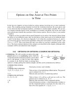
In the last two chapters we have looked at various options involving two or more stochastic
assets. The resulting pricing formulas involved the correlation between the asset prices and
it was observed that in financial markets, correlation is usually highly unstable. We can de-
rive elegant formulas based on the assumption of constant correlation, but in the real world
most practitioners handle these products with extreme caution. However, there is one notable
exception.
Suppose we have an option whose payoff depends on two prices: but instead of these being
the prices of two different assets, they are the prices of the same asset at two different times
τ and T in the future. It is shown in Appendix A.1(vi) that the correlation between S
τ
and S
T
(or to be more precise, between the logarithms of the price movements over the periods τ and
T)isρ =
√
τ/T . This is just about the only case where we can have confidence in the value
for ρ. The most common options in this category are described in this chapter, although other
examples will be encountered in later chapters.
14.1 OPTIONS ON OPTIONS (COMPOUND OPTIONS)
t
T
t
0
now maturity of
underlying
option
time t
maturity

of compound
option
(i) Definitions: We will consider an option (the com-
pound option) on an underlying option. Both the
compound and the underlying options can be either
put or call options, so that we have four options
to consider in all. Half the battle in pricing these
options is simply getting the notation straight, and this can be summarized as follows:
UNDERLYING STOCK:
S
t
and σ Stock price at time t and volatility
UNDERLYING OPTIONS:
C
u
(S
t
, X, t); P
u
(S
t
, X, t)
Value at time t of an underlying call/put option. The general
case is written U (S
t
, X, t)
T ; X Maturity date and strike of underlying options
COMPOUND OPTIONS:
C
C

; P
C
; C
P
; P
P
Value at time t of a call on a call, put on a call, etc. The
general case is written 
U
(S
t
, K , t)
τ ; K Maturity date and strike of the compound options
S
∗
τ
Critical stock price at time τ , which determines whether or
not the compound option is exercised. It is the value of S
τ
that solves the equation K = 
u
(S
∗
τ
, X,τ)
14 Options on One Asset at Two Points in Time
(ii) Payoffs of Compound Options: Before moving on to pricing formulas, it is worth getting an
idea of the likely shape of the curve of the compound price. Let us start with a call on a call. At
time τ , the price of the underlying call is given by the curve shown in Figure 14.1. The payoff
of the compound call option is defined as

C
C
(τ ) = max[C
u
(τ ) − K , 0]
Define S
∗
τ
as the value of S
τ
for which K = C
U
(S
∗
τ
, X,τ). Clearly, the payoff diagram is made
up of the x-axis and that part of the curve C
U
(τ ) which lies above K. This is shown as the solid
line in Figure 14.2, together with the compound option price before maturity (dotted curve).
t
S
*
t
S
Xe
-r (T-t)
K
C
U

(t)
Figure 14.1 Underlying option (call)
t
S
*
t
S
C
U
(t)
U
C(t)
Figure 14.2 Compound option (call on call)
Using the same analysis as for the call on call above, a put option on the underlying stock is
represented by the curve shown in Figure 14.3. The payoff of the compound put option, shown
in Figure 14.4, is
P
P
(τ ) = max[K − P
u
(τ ), 0]
P
U
(t)
t
S
*
t
S
Xe

-r (T-t)
K
Figure 14.3 Underlying option (put)
P
U
(t)
t
S
*
t
S
C
P
(t)
Figure 14.4 Compound option (put on put)
The remaining two compound options have curves shown in Figures 14.5 and 14.6.
(iii) Consider the most common case: a call on a call. In order to calculate the value of this compound
option, we use our well-established methodology of finding the expected value of the payoff in
a risk-neutral world, and discounting to present value at the risk-free rate; but now, the ultimate
payoff is a function of two future stock prices (Geske, 1979):
170
14.1 OPTIONS ON OPTIONS (COMPOUND OPTIONS)
t
S
C
P
(t)
Figure 14.5 Compound option (call on put)
t
S

P
C
(t)
Figure 14.6 Compound option (put on call)
r
S
τ
– The stock price when the compound option matures. If this is less than some critical
value S
∗
τ
, it will not be worth exercising the compound option since the underlying option
would then be cheaper to buy in the market. This may be written
only exercise if S
∗
τ
< S
τ
, where S
∗
τ
is the solution to the equation
K = S
∗
τ
e
−q(T −τ )
N[d
∗
1

] − X e
−r(T −τ )
N[d
∗
2
]
d
∗
1
and d
∗
2
are the usual Black Scholes parameters with the stock price set equal to S
∗
τ
.
r
S
T
– The stock price when the underlying option matures. The ultimate payoff at time T is
the payoff of the underlying call, if (and only if) the condition S
∗
τ
< S
τ
was fulfilled. This
ultimate payoff is of course a function of S
T
.
Since the value of a compound option depends on the expected values of both S

τ
and S
T
,we
must examine their joint probability distribution.
(iv) Following the approach of Section 5.2(i) for the Black Scholes formula, the price of this option
may be expressed as
C
C
(0) = PV

E

payoff of underlying option
−payment for underlying option



only if compound
option was exercised

risk neutral

r
“Only if compound option exercised” ≡ S
∗
τ
< S
τ
.

r
“Payment for underlying” = K at time τ .
r
“Payoff of underlying option” (at time T) = max[0, S
T
− X].
Combining this together and simplifying the notation gives
C
C
(0) = e
−rT
E[max[S
T
− X, 0]: S
∗
τ
< S
τ
] − e
−rτ
E[K : S
∗
τ
< S
τ
]
= e
−rT
E[S
T

− X : S
∗
τ
< S
τ
; X < S
T
] − e
−rτ
K P[S
∗
τ
< S
τ
] (14.1)
These expectations are evaluated explicitly in Appendix A.1(v) and (ix), to give
C
C
(0) = S
0
e
−qT
N
2
[d
1
, b
1
; ρ] − X e
−rT

N
2
[d
2
, b
2
; ρ] − K e
−rτ
N[b
2
] (14.2a)
171
14 Options on One Asset at Two Points in Time
where
d
1
=
1
σ
√
T

ln
S
0
e
−qT
X e
−rT
+

1
2
σ
2
T

; b
1
=
1
σ
√
τ

ln
S
0
e
−qτ
S
∗
τ
e
−rτ
+
1
2
σ
2
τ


d
2
= d
1
− σ
√
T ; b
2
= b
1
− σ
√
τ ; ρ =

τ
T
and S
∗
τ
is a solution to the equation K = C
U
(S
∗
τ
, X,τ). The lower limits of integration in
the above-mentioned appendices are the values of z
τ
and z
T

corresponding to S
τ
= S
∗
τ
and
S
T
= X .
(v) General Formula: The put–call parity relationship
C
C
(0) + K e
−rτ
= P
C
(0) + C
U
(0)
may be used to calculate the formula for a put on an underlying call. The relationships
N[d] + N[−d] = 1 and N
2
[d, b; ρ] + N
2
[d,−b;−ρ] = N[d] [see equation (A1.17)] are used
to simplify the algebra, giving
P
C
(0) = X e
−rT

N
2
[d
2
,−b
2
;−ρ] − S
0
e
−qT
N
2
[d
1
,−b
1
;−ρ] + K e
−rτ
N[−b
2
]
Similar results are obtained for put and call options on an underlying put option. The four
possibilities for compound options can be summarized in the general formula

U
(0) = φ
U
φ

{S

0
e
−qT
N
2
[φ
U
d
1
,φ
U
φ

b
1
; φ

ρ] − X e
−rT
N
2
[φ
U
d
2
,φ
U
φ

b

2
; φ

ρ]}
− φ

K e
−rτ
N[φ
U
φ

b
2
] (14.2b)
where
d
1
=
1
σ
√
T

ln
S
0
e
−qT
X e

−rT
+
1
2
σ
2
T

; b
1
=
1
σ
√
τ

ln
S
0
e
−qτ
S
∗
τ
e
−rτ
+
1
2
σ

2
τ

d
2
= d
1
− σ
√
T ; b
2
= b
1
− σ
√
τ ; ρ =

τ
T
; S
∗
τ
solves K = 
U
(S
∗
τ
, X,τ)
φ
U

=

+1 underlying call
−1 underlying put
φ

=

+1 compound call
−1 compound put
(vi) Installment Options: When they are first encountered, compound options often look to stu-
dents like rather contrived exercises in option theory. However they do have very practical
applications, as the following product description indicates:
r
An investor receives a European call option which expires at time T and has strike X.
r
Instead of paying the entire premium now, the investor pays a first installment of C
C
today.
r
At time τ , the investor has the choice of walking away from the deal or paying a second
installment K and continuing to hold the option.
This structure clearly has appeal in certain circumstances; it is just the call on a call described
in this section, but couched in slightly less dry terms.
172
14.2 COMPLEX CHOOSERS
14.2 COMPLEX CHOOSERS
Recall the simple chooser which was described in Section 11.2: we buy the option with strike
X at time t = 0 and at t = τ we decide whether the option which matures at t = T is a put
or a call. The complex chooser is similar in principle, but the put and call can have different

maturities and strikes (Rubinstein, 1991b). The payoff at time τ is therefore written
Payoff
τ
= max[C(S
τ
, X
C
, T
C
− τ ), P(S
τ
, X
P
, T
P
− τ )]
For some critical price S
∗
τ
at time τ , the value of the put and the call are exactly the same. S
∗
τ
is obtained from the equation
C(S
∗
τ
, X
C
, T
C

− τ ) = P(S
∗
τ
, X
P
, T
P
− τ ) (14.3)
using some numerical procedure or the goal seek function of a spread sheet. For S
τ
< S
∗
τ
, the
payoff is the put option, while for S
∗
τ
< S
τ
the call option price is larger. Using the reasoning
of Section 14.1(iv) gives
f
complex chooser
= e
−rT
C
E

S
T

C
− X
C


S
∗
τ
< S
τ
; X
c
< S
T
C

+ e
−rT
P
E

X
P
− S
T
P


S
τ

< S
∗
τ
; S
T
P
< X
P

The first term here is just the first term of equation (14.1) for a call on a call; similarly, the
second term is the first term of the formula for a call on a put. Instead of slogging through a
bunch of double integrals again, we just steal the answer from equation (14.2b):
f
complex chooser
=

S
0
e
−qT
C
N
2

d
(C)
1
, b
1
; ρ

(C)

− X
C
e
−rT
C
N
2

d
(C)
2
, b
2
; ρ
(C)

−

S
0
e
−qT
P
N
2

−d
(P)

1
,−b
1
; ρ
(P)

− X
P
e
−rT
P
N
2

−d
(P)
2
,−b
2
; ρ
(P)

(14.4)
d
(i)
1
=
1
σ
√

T
i

ln
S
0
e
−qT
i
X
i
e
−rT
i
+
1
2
σ
2
T
i

, i = C or P; b
1
=
1
σ
√
τ


ln
S
0
e
−qτ
S
∗
τ
e
−rτ
+
1
2
σ
2
τ

S
∗
τ
solves equation (14.3):
d
(i)
2
= d
(i)
1
− σ

T

i
; b
2
= b
1
− σ
√
τ ; ρ
(i)
=

τ
T
i
14.3 EXTENDIBLE OPTIONS
(i) Consider a European call option with maturity at time τ and strike price K; at maturity, the
holder has the choice of exercising or not exercising (Longstaff, 1990). Now suppose that
an additional feature is added to this option: the holder is given a third choice at maturity of
extending the option to time T at a new strike price X, in exchange for a fee of k. The payoff
of this extendible option at time τ is
max[0, S
τ
− K, C(S
τ
, X, T − τ) − k]
The issues are best illustrated graphically. Figure 14.7 shows the value of the extended call
option C(S
τ
, X, T − τ) at time τ . This is just a simple graph of a European call option at time
173