Numerical Solutions of the Black Scholes Equation
Bạn đang xem bản rút gọn của tài liệu. Xem và tải ngay bản đầy đủ của tài liệu tại đây (354.99 KB, 18 trang )
8
Numerical Solutions of the Black
Scholes Equation
8.1 FINITE DIFFERENCE APPROXIMATIONS
(i) The object of this chapter is to explain various methods of solving the Black Scholes equation
by numerical methods, and to relate these to other approaches to option pricing. We start with
the Black Scholes equation in the following form:
∂ f
0
∂T
= (r − q)S
0
∂ f
0
∂ S
0
+
1
2
S
2
0
σ
2
∂
2
f
0
∂ S
2
0
− rf
0
(8.1)
where S
0
and f
0
are the prices of the stock and derivative at a time T before maturity. Using
equation (A3.4) of the Appendix, this can be written as a heat equation
∂u
∂t
=
∂
2
u
∂x
2
(8.2)
where
f
0
(S
0
, T ) = e
−rT
(e
−kx−k
2
t
u(x, T )); x = ln S
0
; t =
1
2
σ
2
T ; k =
r − q −
1
2
σ
2
σ
2
We depart from our usual practice of saving the symbol t for time (in the sense of date),
although T remains time (to maturity). This saves us having to use obscure or non-standard
symbols and should be unambiguous.
(ii) The solution u(x , t) can be envisaged as a three-dimensional surface over the (x , t) plane.
The values of x range from −∞ to +∞, and the values of t from 0 to +∞. Imagine that we
cover the x–t plane with a discrete set of equally spaced grid points, which are δx apart in
the x-direction and δt apart in the t-direction, as shown in Figure 8.1. At the grid points, we
can write x = mδx and t = nδt, where m and n are integers. The coordinates of a grid point
can therefore be defined by counting off grid lines from the origin. The notation we adopt for
u(x, t) at a grid point is
u(x, t) = u(mδx, nδt) = u
n
m
(iii) A first-order approximation of the right-hand side of the heat equation can be written as
∂
2
u
∂x
2
=
∂
∂x
∂u
∂x
→
1
δx
1
δx
u
n
m+1
− u
n
m
−
u
n
m
− u
n
m−1
=
1
(δx)
2
u
n
m+1
+ u
n
m−1
− 2u
n
m
≡
1
(δx)
2
ˆ
δ
2
x
u
n
m
where the operator
ˆ
δ
2
x
is defined by the last identity, and will be used in the interests of brevity.
This approximation is symmetric in u
n
m
and there is no reason to assume that it is subject to
any bias.
8 Numerical Solutions of the Black Scholes Equation
The left-hand side of the heat equation, on the other hand, cannot be unambiguously ap-
proximated. The following are some of the more common approximations, whose merits are
discussed later.
0
1
u
0
0
u
0
1
u
−
1
0
u
0
2
u
n+1
u
m
n+1
u
m−1
n
u
m+1
n+1
u
m+1
n
u
m
n
u
m−1
Figure 8.1 Discretization grid
(iv) Forward Difference:
∂u
∂t
=
1
δt
u
n+1
m
− u
n
m
This is the most obvious approximation, but clearly introduces a bias since it is not centered
on the time grid points, but half way between n and n + 1. Using this approximation, the heat
equation gives the following finite difference equation:
u
n+1
m
− u
n
m
= α
ˆ
δ
2
x
u
n
m
= α
u
n
m+1
+ u
n
m−1
− 2u
n
m
where α =
δt
(δx)
2
(v) Backward Difference:
∂u
∂t
=
1
δt
u
n
m
− u
n−1
m
This looks similar to the forward difference method, except that it is centered half way between
time grid points n − 1 and n, so that the bias is in the opposite direction. The resulting difference
equation is
u
n
m
− u
n−1
m
= α
ˆ
δ
2
x
u
n
m
= α
u
n
m+1
+ u
n
m−1
− 2u
n
m
(vi) Richardson: The previous two methods cause forward and backward biases on the time axis,
so a simple remedy might be to take the average of the two:
1
2
u
n+1
m
− u
n−1
m
= α
ˆ
δ
2
x
u
n
m
= α
u
n
m+1
+ u
n
m−1
− 2u
n
m
This seems an appealing solution; but the Richardson method is a standard textbook example
of how simple intuitive solutions do not always work. The method has a hidden defect which
makes it unusable, as described below.
(vii) Dufort and Frankel: This is an attempt to adapt the Richardson method so that it eliminates
bias (but also works!). We simply replace the final term u
n
m
in the Richardson scheme by the
88
8.2 CONDITIONS FOR SATISFACTORY SOLUTIONS
average of u
n+1
m
and u
n−1
m
, giving
1
2
u
n+1
m
− u
n−1
m
= α
u
n
m+1
+ u
n
m−1
−
u
n+1
m
+ u
n−1
m
= α
ˆ
δ
2
x
u
n
m
− α
u
n+1
m
+ u
n−1
m
− 2u
n
m
This method does in fact work, although not especially well, and we will see below that if we
are careless in applying the scheme it can lead to quite spurious answers.
(viii) Crank Nicolson: This is the most important scheme, and the one that the reader is likely to
use if he is going to use the finite difference method seriously. The last two methods tried to
overcome the biases which are inherent in the discretization of the time variable. However,
there is another approach: when using the approximation for ∂
2
u/∂ x
2
, use the average of the
values at n and n + 1. The result is simply
u
n+1
m
− u
n
m
=
1
2
α
ˆ
δ
2
x
u
n+1
m
+ u
n
m
This could be regarded simply as the average of the forward difference result, and the backward
difference result one time step later.
(ix) Douglas:
u
n+1
m
− u
n
m
=
1
2
α
ˆ
δ
2
x
1 −
1
6α
u
n+1
m
+
1 +
1
6α
u
n
m
Where on earth did this come from? There is no simple intuitive explanation, but the really
interested reader will find the derivation in Section A.9 of the Appendix. This scheme takes
just about the same effort to implement as Crank Nicholson but can be much more accurate. It
can be shown that it is at its most accurate if we put α = 1/
√
20. Note that if we put α = 1/6,
the difference equation reduces to the forward difference scheme described above.
8.2 CONDITIONS FOR SATISFACTORY SOLUTIONS
The six schemes set out in the last section all seem quite reasonable; but are there any tests we
can carry out ahead of time, to check that we get sensible answers? It turns out that there are
three conditions that must be met which are explained below; but before turning to these, it is
worth pointing out to the reader that the numerical solution of partial differential equations is
something of an art form, containing many hidden pitfalls. We explain the principles behind
the three conditions, but we will not elaborate on the precise techniques used in testing for the
conditions. The reader can perfectly well use the discretizations described, taking on trust the
comments we make on their applicability. Alternatively, if he wants to be more creative and
devise new discretizations, he will have to delve into the subject more deeply than this book
allows.
(i) Consistency: In simple terms, we must make sure that as the grid becomes finer and finer,
the difference equation converges to the partial differential equation we started with (the heat
equation), and not some other equation. This may sound rather fanciful, so let us take a closer
look at the Dufort and Frankel scheme. On the face of it, we have merely eliminated the biases
of the forward and backward methods, without any very fundamental change. But in the limit
89
8 Numerical Solutions of the Black Scholes Equation
of an infinitesimally fine grid, we may write
1
2
u
n+1
m
− u
n−1
m
→ δt
∂u
∂t
; α
ˆ
δ
2
x
u
n
m
→ α(δx)
2
∂
2
u
∂ x
2
α
u
n+1
m
+ u
n−1
m
− 2u
n
m
→ α(δt)
2
∂
2
u
∂t
2
so that the equation for the Dufort–Frankel scheme in Section 8.1(vii) becomes
∂u
∂t
+ β
2
∂
2
u
∂t
2
=
∂
2
u
∂ x
2
; β =
δt
δx
If we decrease the grid size at the same rate in the x- and t-directions (i.e. keep β constant),
the Dufort and Frankel scheme converges to a hyperbolic partial differential equation, which
is quite different from the heat equation. On the other hand, if we decrease the mesh in such
a way that α = δt/(δx)
2
= constant, β would tend to zero and the finite difference equation
would be consistent with the heat equation. This constant α convergence is in fact the most
common way for progressively making the grid finer.
(ii) Convergence: This concept is easy to describe: does the value obtained by solving the difference
equation converge to the right number as δx, δt → 0? Or converge to the wrong number
(inconsistent), or oscillate or just wander about indefinitely? Unfortunately, precise tests for
convergence are difficult to devise. We therefore move on quickly, and later discover that there
is a round-about way of avoiding the whole issue.
(iii) Stability: Suppose we have set up some discretization scheme to solve the heat equation; we
have calculated all the numbers by hand to four decimal places and are satisfied with the
answers. But as a quick last check, we decide to run all the numbers again to one decimal
place. To our dismay, we get a substantially different answer. Does this mean that we made
an arithmetical slip somewhere? Unfortunately, the answer is “not necessarily”. It is in the
nature of some discretization schemes that as we move forward in time, a small initial error
gets magnified at each step and may eventually swamp the underlying answer. Such a scheme
is said to be unstable.
The underlying test we must make of any scheme with N time steps of length δx is to let
N →∞and δt → 0 in such a way that N δt = t remains finite, and then see if a small error
introduced at t = 0 could become unbounded by the time it is transmitted to time step N. There
are two commonly used tests for stability which are quite simple to apply. However, we content
ourselves here with merely giving results for the schemes we introduced in the last section.
r
The forward difference method is stable only if α ≤
1
2
.
r
The backward difference, Crank Nicholson and Douglas methods are always stable.
r
The Richardson method is always unstable.
r
Dufort and Frankel is always stable but as we saw above, it may not be consistent with the
heat equation.
(iv) Lax’s Equivalence Theorem: The reader might feel we have tip-toed away from the con-
vergence issue raised in subparagraph (ii) above. However, this theorem states that subject
to some technical conditions, stability is both a necessary and sufficient condition to assure
convergence, i.e. if we have got the stability conditions right, we can forget about convergence.
90
8.3 EXPLICIT FINITE DIFFERENCE METHOD
Conversely, if a stability condition is even slightly broken, the solutions may fail to converge
in quite a dramatic way; an example of this is given later.
8.3 EXPLICIT FINITE DIFFERENCE METHOD
(i) The forward difference scheme of Section 8.1(iv) can be written
u
n+1
m
= (1 − 2α)u
n
m
+ α
u
n
m+1
+ u
n
m−1
; α =
δt
(δx)
2
≤
1
2
n+1
u
m+1
n
u
m+1
n
u
m
n
u
m−1
n+1
u
m
n+1
u
m−1
Figure 8.2 Forward difference
This is represented in Figure 8.2, which shows a small
part of the total grid. The key point to notice is that each
u
n+1
m
can be calculated from the three values of u to the
immediate left, by simple arithmetic combination.
In general, when we use a finite difference method
to solve the heat equation, we start off knowing all the
values for t = 0 along the vertical axis; these are the
initial conditions. We also know the grid values for
certain values of x when t > 0; these are the boundary
conditions. For simple options they consist of known
values of u
n
m
as x approaches ±∞.
If the forward finite difference scheme is used to calculate a particular value for u(x , t) = u
N
M
,
we start with the initial values at t = 0 and work across the grid towards the point (N, M).
But because of the simple way in which the u
n+1
m
only depend on the adjacent values to the
immediate left, only solutions within the shaded area of Figure 8.3 need to be calculated. This
leads to the slightly surprising conclusion that the boundary conditions are redundant.
This method is called the explicit difference method because we start with a knowledge of
the u
0
m
at the left-hand edge and can explicitly work out any u
n
m
from these.
Initial Conditions
only these affect answer
explicit solutions
Answer
x =+∞
x =−∞
t = 0
Figure 8.3 Explicit method
91
8 Numerical Solutions of the Black Scholes Equation
(ii) We are free to choose whatever value for α we please, subject to the scheme conforming
with the stability conditions. If we choose α =
1
2
, the finite difference equation becomes even
simpler:
u
n+1
m
=
1
2
u
n
m+1
+ u
n
m−1
subject to grid spacing δx =
√
2δt
This scheme looks suspiciously like a binomial model turned back to front. But such a re-
versal is purely a question of conventions for assigning time. In the conventions of the heat
equation, t = 0 means “at the beginning” in a calendar sense; this is when the initial con-
ditions (temperature distribution in a long thin conductor) are imposed. In option theory, T
means time left to maturity; therefore T = 0 means “at maturity”. This is why the payoff
of an option (value at maturity) is often confusingly referred to as the initial conditions. In
Figure 8.3 we can flip the triangular network so that the initial conditions are on the right and
the “answer” is at the apex of the triangle on the left. But this now looks just like a binomial
tree.
(iii) Equivalence of Binomial Tree and Explicit Finite Difference Method: Let us return to equa-
tion (8.2) to see how this simple two-pronged discretization scheme looks when expressed in
terms of the underlying stock price, rather than its logarithm. The grid spacing relationship
becomes
δx = x
n
m+1
− x
n
m
= ln
S
m+1
S
m
=
√
2δt = σ
√
δT
or more simply
S
m+1
= S
m
e
σ
√
δ
T
Similarly, we may write
u
n+1
m
= e
r(T+
δ
T )
e
kx+
1
2
k
2
σ
2
(T+
δ
T )
f
n+1
m
u
n
m+1
= e
rT
e
k(x+
δ
x)+
1
2
k
2
σ
2
T
f
n
m+1
u
n
m−1
= e
rT
e
k(x−
δ
x)+
1
2
k
2
σ
2
T
f
n
m−1
Substituting these into the binomial scheme gives the relationship
f
n+1
m
= e
−r
δ
T
1
2
e
λ+
1
2
λ
2
f
n
m+1
+
1
2
e
λ−
1
2
λ
2
f
n
m−1
λ = kσ
√
δT
Expanding the exponentials and discarding terms of O[δt
3/2
] leads to
f
n+1
m
= e
−r
δ
T
pf
n
m+1
+ (1 − p) f
n
m−1
p =
1
2
+
1
2
r − q −
1
2
σ
2
σ
√
δT
This is precisely the Jarrow–Rudd version of the binomial model, summed up in equation (7.6).
The binomial model and the explicit finite difference solution of the Black Scholes equation
are simply different ways of expressing the same mathematical formalism. This conclusion
is reinforced by the essential stability condition α ≤
1
2
mentioned in Section 8.2(iii); again
92
8.4 IMPLICIT FINITE DIFFERENCE METHODS
discarding terms of O[δt
3/2
], this may be written in terms of T and S
T
as S
T
σ
√
δT /2δS
T
≤
1
2
.
To the present order of accuracy in δT , this is the same condition that was expressed by
equation (7.4), and which came from a seemingly unrelated line of reasoning.
This should of course be of no great surprise:
r
The binomial model is a graphical way of approximating the probability density function of
a stock price (or its logarithm).
r
This probability density function is a solution of the Kolmogorov backward equation; there-
fore the binomial model is a graphical representation of the Kolmogorov equation.
r
The explicit difference method was introduced to solve the Black Scholes equation.
r
The Kolmogorov and Black Scholes equations are shown in Section A.4(i) of the Appendix
to be very closely related.
This duality between the explicit finite difference method and the binomial model is also true
of the trinomial model which is examined in a later chapter.
8.4 IMPLICIT FINITE DIFFERENCE METHODS
(i) Let us return to the backward difference scheme of Section 8.1(v) which may be written
u
n−1
m
= (1+ 2α)u
n
m
− α
u
n
m+1
+ u
n
m−1
n+1
u
m+1
n+1
u
m
n+1
u
m−1
n
u
m−1
n
u
m
n
u
m+1
Figure 8.4 Backward difference
and which is represented in Figure 8.4. In this case u
n−1
m
can be calculated from the adjacent u values immedi-
ately to the right. Unfortunately, this is an inconvenient
way to proceed. We know the values at the left-hand
edge of the grid (initial conditions) and the values at
the top and bottom edges (boundary conditions); the
solution of the problem is the series of values at the
right-hand edge. In order to find these right-hand edge
solutions, we need to solve a large array of linear si-
multaneous equations for all the u
n
m
; these are not
given explicitly in terms of known quantities – hence the name implicit methods.
(ii) As well as producing awkward simultaneous equations to solve, the implicit difference intro-
duces difficult boundary conditions. Compare Figures 8.3 and 8.5, showing boundary con-
ditions for the two methods. The simple nature of the explicit difference method meant that
we could ignore all values outside the shaded area, including boundary values. But with the
implicit method, boundary values are important.
For a European call option the boundary conditions are
lim
S
0
→∞
f
0
(S
0
, T ) → S
0
e
−qT
− X e
−rT
lim
S
0
→0
f
0
(S
0
, T ) = 0
93