Bài báo cáo thực hành 1 môn lý thuyết mạch (Circuit Theory)
Bạn đang xem bản rút gọn của tài liệu. Xem và tải ngay bản đầy đủ của tài liệu tại đây (2.08 MB, 18 trang )
The University of Danang
Danang University of Science and Technology
Contents
Step Response of RC Circuits
1.
2.
3.
4.
Objectives………………………………………………………
Reference……………………………………………………….
Circuits…………………………………………………………
Components and
specifications………………………………..
LAB REPORT
Instructor
: Nguyen Tri Bang
Lab
:1
Class
: 15ECE2
Group members: Tran Viet Tu
Nguyen Cong Thien
Dinh Ngoc Tien
Le Dinh Hoai Nam
Danang 2017
Danang 2017
Step Response of RC Circuits
1. Objectives
Measure the internal resistance of a signal source (e.g. an arbitrary
waveform generator).
Measure the output waveform of simple RC circuits excited by step
functions.
Calculate and measure various timing parameters of switching
waveforms (time constant, delay time, rise time, and fall time)
common in computer systems.
Compare theoretical calculations and experimental data, and explain
any discrepancies.
2. Reference
The step response of RC circuits is covered in the textbook. Review
the appropriate sections, look at signal waveforms, and review the
definition and formula for the time constant.
Review the usage of laboratory instruments.
3. Circuits
Figure 1 shows a simple circuit of a function generator driving a resistive load. This
circuit is used to illustrate and measure the internal resistance of a function generator.
Figure 2 shows the first-order RC circuit whose step response will be studied in this lab.
Figure 3 shows two sections of the first-order RC circuit connected in series to
illustrate a simple technique to model computer bus systems (PCI bus, SCSI bus, etc.).
4. Components and Specifications
Quantity
Descriptions
Comments
1
50 Ω resistor
Real value : 50.42 Ω
2
10 KΩ resistor
Real value : 9.98 kΩ
1
27 KΩ resistor
Real value : 27.30 kΩ
2
0.01 μF capacitor
Real value : 0.01μF
capacitor
-
-
5. Experimental proceduces:
5.1
Instruments needed for this experiment
An arbitrary waveform generator.
A multimeter.
A board and an oscilloscope.
5.2
Effects of internal resistance of function generator
1. Build the circuit in Figure 1 using a 50 Ω resistor as load. Set the
function generator to provide a square wave with amplitude 400
mV, DC offset 0V, and frequency 100 Hz.
2. Use the scope to display the signal Vout on channel 1, using DC
coupling. Set the horizontal
Time base to display 3 or 4 complete cycles of the signal.
3. Use the scope to measure the amplitude of Vout. Record this value
in your report. Is it the same as the amplitude displayed by the
function generator? Explain any difference.
- The amplitude of is = 160 (mV).
* It is smaller than the amplitude displayed. The reason is that the
voltage is dropped by the internal resistor Rs of the generator.
4. Vary the square wave amplitudes from 400 mV to 1 V, using 100
mV step size (e.g. the amplitudes are 400 mV, 500 mV up to 1 V).
Repeat step 3 to measure the amplitude of Vout on the scope for
each setting. Get a hardcopy for the case of 500 mV amplitude only.
6. Remove the 50 Ωresistor and replace it with a 27 KΩresistor.
Repeat the steps 1 through 4 above. Observe and explain any
difference insignal amplitudes when the loading on the function
generator is changed from50 Ω to 27 KΩ.
Source
Amplitu
de
-
400
401
500
539
600
610
700
715
800
820
900
925
1000
1020
When R1= 27 kOhm, we can see that the value of Vout equals
to the value of Vin.
Source (mV)
400 500 600 700 800 900 1000
Amplitude (mV)
100 125 150 174 204 228
254
- When the loading on the function generator is changed to 27 ,
the inaccuracy of signal amplitudes is very small. Thus, the
output voltage is approximately the input voltage.
-
7.3
. When using the formula in the prelab 1, since R1 >> R s, we
can consider that Rs is approximately zero. Therefore, the value
of Vout is equal to the value of Vin. In other words, when the
value of R1 >> value of Rs, the value of Vout is not be affected
by the value of the internal resistance of the generator.
Step response of first-order RC circuits
1. Build the circuit in Figure 2 using R = 10 KΩ and C = 0.01 μF. Set
the arbitrary waveform generator provide a square wave input as
follows:
a. Frequency = 300 HZ (to ensure that T >> RC, T=1/f). This value
of frequency guarantees that the output signal has sufficient time to
reach a final value before the next input transition.
b. Set the Amplitude from 0 V to 5.0 V.
Note that you need to set
the offset to achieve this waveform. Use the oscilloscope to display
this waveform on Channel 1 to make sure the amplitude is correct.
We use this amplitude since it is common in computer systems.
c. Set both channel 1 and channel 2 to DC coupling.
2. Use Channel 2 of the
oscilloscope to display the
output signal waveform. Adjust
the timebase to display 2
complete cycles of the signals.
Record the maximum and the
minimum values of the output
signal
Vout Max=4.98V Vout min = 0
V
3.Use
the
capability of
measurement
the scope to
measure the period T of the input signal, the time value of the 10%point of Vout, the time value of the 90%-point of Vout, and the time
value of the 50%-point of Vout
The
time value of the 10%-point of Vout
Period of input = 3.000 ms
Rise time: the time interval between the 10%-point and the
90%-point of the waveform when thesignal makes the
transition from low voltage (L) to high voltage (H).
= 290 µs
Fall time: the time interval between the 90%-point and the
10%-point of the waveform when thesignal makes the
transition from high voltage (H) to low voltage (L).
= 304 µs
= 68.0 µs
= 56.0 µs
4. Save a screenshot from the display with both waveforms and the
measured values.
5. Measure the rise time of Vout, the fall time of Vout, and the two
delay times tPHL and tPLH between the input and output signals.
6. Save a screenshot from the display with both waveforms
and the measured values.
7. Measure the voltage and time values at 10 points on the
Vout waveform during one interval when Vout rises or falls with
time (pick one interval only). Note that the time values should be
referred to time t = 0 at the point where the input signal rises from 0
V to 5 V or falls from 5 V to 0 V. Record these 10 measurements.
Time 16 μs 20 μs 22 μs 36 μs 42 μs 48 μs 108 μs134 μs190 μs240 μs
Voltage
638
mV
790
mV
1.1 V 1.4 V 1.6 V 1.8 V
3V
3.4 V
4 V 4.32 V
7.4 Step response of cascaded RC sections
1. Build the circuit in Figure 3, using 2 identical resistors R = 10 KΩ
and 2 identical capacitors C =0.01 µF. Use the same square input as
in item 1, section 7.3 above and display it on Channel 1
2. Display Vout on Channel 2 and adjust the time base to display 2
complete cycles of the signal
Use the scope measurement capability to measure the two delay
times tPHL and tPLH between the input and output signals
tPHL = 220 μs
= 260 µs
7.5 Manufacturing test time and test cost considerations
1. The more points you measure on a waveform, the more
accurate the measured results but this also takes more time
and increases the test cost. This is an important tradeoff in
measurement accuracy and test cost. Given the circuit in
Figure 2, ten data points per waveform were collected in
section 7.3 item 7. “Good” estimate means the estimated
value is within 10% of the correct value (from computation or
simulation).
We should collect more than 10 points to extract a “good”
estimate of the rise or fall time of the circuit
2. The minimum number of data points do you need to collect to
get a good estimate is 15. Other teams collect fewer points.
We think their results are not “better” than ours.
2500
2000
1500
1000
500
0
0
500
1000
1500
2000
2500
3000
3500
8. Analysis, calculation and results (Tabulated data) and
answers to questions:
8.1
Extracting internal resistance of an arbitrary
waveform generator
1. Vout = R1/(R1+Rs) * Vs
R1 = 50 Ω Vout = 50/(50+50) * 500 = 250 (mV)
R1= 27 kΩ Vout = 2700/(2700+50) * 500 = 499.07 (mV)
This value doesn’t agree with the recorded data in the lab.
2 From the data recorded in section 7.2 : Rs=50Ω
3 The values for Vs (as displayed by an arbitrary waveform
generator panel) and the measured values on the scope are
not the same.Because of the resistor of the wire and the
generator is not ideal.
8.2
1 R = 10.013 kΩ. C=0.01 µF.
Vout = Vs (1 - e –t/RC)
Vs = 5 (V) when t = T Voutmin= 0 (mV) when t = 0
Voutmax(measured) = 4.96V < 5V due to the existence of sources
internal resistance.
2
Calculated value
10.53 μs
0->10%: Δt1 = -RC.ln
0.9
0->50%: Δt2 = -RC.ln
69.31 μs
0.5
0->90%: Δt3 = -RC.ln
230.25 μs
0.1
Error: 0->10% : 5.03%
Measured value
10 μs
80 μs
280 μs
0->50% : 15.42%
0->90% : 21.6%
Because the source has internal resistance so R eq = Rs + R > R
so t in practical is larger than t in theory.
3
tfall= trise = Δt3 - Δt1
Calculated value
219.72μs
tPHL=tPLH= Δt2
69.31μs
Measured value
trise=270 μs, tfall= 260
μs
80 μs
The internal resistance is the sources of errors leading to the
differences.
Error is committed by neglecting the internal resistance of the
arbitrary waveform generator: t rise: 22.88%
tfall :18.33%
tPHL and tPLH :15.42%
4
Time 16 μs 20 μs
Voltag 720
e
mV
22 36 42 48 108 134 190 240
μs μs μs μs μs μs μs μs
880
1.4 1.6 1.8
4.32
1V
3 V 3.4 V 4 V
mV
V V V
V
(Ƭ is time constant)
Ƭ=RC=0.0001s
Ƭ measured:0.000104658s
The difference in percent: 4.658%
.
5
(Ƭ is time constant)
Ƭ=RC=0.0001
Ƭ measured : 0.000110494s
The difference in percent with 4: 10.494 % greater than
4.658%
Ƭ=RC therefore C= Ƭ/R= 0.011035 µF this value greater than
the marked value
8.3
1 For the measurements in section 7.4 item3, the delay time for
the cascaded circuit in Figure 3 ( of 2 identical RC sections) are
not twice as large as the delay times for the simple RC circuit.
The delay time scale with the number of sections.
We have
Vc1 = VR + Vc2
Taking the derivative both sides, we obtain: dVc1/dt =
dVc2/dt
We also have:
Is = Ic1 + Ic2
Vs/R = C1 dVc1 / dt + C2dVc2 / dt
C1 = C2 = C => Vs= 2RC * dV2/dt = 2RC
dVout/dt
=> Ƭ =1/2 RC
The expression of t: t = -2RC * ln(1 – Vout/Vs)
In section 7.3, we have: t = -RC * ln(1 – Vout/Vs)
So it is easy to show that the delay time for the cascaded
circuit (in Figure 3) is double the delay time for the simple RC
circuit. Similarly, we can show this problem for n sections:
t =n* ( -RC * ln(1 – Vout/Vs))
2 The number of cascaded RC sections so that the propagation
delay time is about T/2
Tdelay = T/2 n* ( -RC * ln(1 – Vout/Vs)) = T/2 =1/(2f)
n = -1/(2RCf * ln(1 - Vout/Vs))
With delay time, we have Vout/Vs = 0.5. in section 7.3, we
have R = 10kΩ, C=0.01µF
n = 24 sections.
According to the delay time measured at the Figure 5:
tdelay.1 = 76 µs of one RC section (in Figure 1).
With n sections, we have tdelay.n= n*tdelay.1 n = tdelay.n/tdelay.1
With tdelay.n = T/2=1/2f=1/600(s).
Therefore, n=1/(600*76*10-6)=22
%errors = 8.3% < 10%.So this is a good estimate.
CONCLUSION:
This report has discussed the output waveform of simple RC circuits
excited by step functions, timing parameters of switching waveform
conclude time constant, delay time, rise time, and fall time. The
differences between theoretical calculations and experimental data
are significant. The data collected correlated strongly to the
hypotheses, although percent errors reaching high value ( largely
>15%) because the internal resisters have influence on measured
results.
Furthermore,
the
differences
between
theoretical
calculations and experimental data due to the mechanical error.