HIỆN TƯỢNG ĐIỆN ĐỘNG HỌC TRONG ỐNG MAO DẪN HÌNH TRỤ
Bạn đang xem bản rút gọn của tài liệu. Xem và tải ngay bản đầy đủ của tài liệu tại đây (468.59 KB, 7 trang )
<span class='text_page_counter'>(1)</span><div class='page_container' data-page=1>
<b>ELECTROKINETICS IN A CYLINDRICAL CAPILLARY </b>
<b>Luong Duy Thanh1,*, Phan Van Do1, Pham Thi Thanh Nga1, </b>
<b>Nguyen Trong Tam2, Pham Thi Na3, Phan Thi Ngoc3 </b>
<i>1<sub>Thuyloi University, </sub>2<sub>Vietnam Maritime University, </sub></i>
<i>3</i>
<i>University of Science - TNU </i>
ABSTRACT
Electrokinetic phenomena are induced by the relative motion between a fluid and a solid surface
and are directly related to the existence of an electrical double layer with excess charges. In this
work, we use a theoretical study of electrokinetics in a narrow cylindrical capillary to obtain the
streaming potential and electroosmosis coefficients under the thin double layer assumption. We
<i>use the obtained theoretical coefficients to compare with experimental data available in literature. </i>
The results show a good agreement between the theory and the experimental data and that
validates the obtained model. The model for a narrow cylindrical capillary is a basis to understand
electrokinetics in porous media.
<i><b>Keywords: electrokinetics, zeta potential, porous media, electric double layer, </b></i>
INTRODUCTION*
Electrokinetic phenomena consist of different
effects such as streaming potential,
electroosmosis etc. When the pore fluid is
mechanically forced to flow through a porous
media, some of the excess charges are
dragged to move, therefore causing streaming
electric current in porous media, which is
referred to as the streaming potential effect
(SP). Conversely, an applied electric field
forces the excess charges to move, therefore
driving pore fluid flow, which is referred to as
the electroosmosis effect (EO).
Electrokinetics plays an important role in
geophysical applications, environmental
applications, medical applications and other
applications. For example, SP measurement is
used to detect subsurface flow in oil
reservoirs or to monitor subsurface flow in
geothermal areas and volcanoes. It is also
used to detect seepage of water through
retention structures such as dams, dikes, and
canals etc. [1]. SP has been utilized to
generate electric power by pumping liquids
such as tap water through tiny micro channels
[2,3]. EO is one of the promising technologies
for cleaning up low permeable soil in
*
<i>Email: </i>
environmental applications. In this process,
the contaminants are separated by the
application of an electric field between two
electrodes inserted in contaminated masses.
Therefore, it has been used for the removal of
organic contaminants, heavy metals,
petroleum hydrocarbons etc. in soils, sludge
and sediments. Additionally, EO has been
used to produce microfluidic devices such as
EO pumps with several outstanding features:
ability of generating constant and pulse-free
flows, facility of controlling the flow
magnitude and direction of EO Pumps, no
moving parts. EO Pumps have been used in
microelectronic equipment for drug delivery
etc [4].
<i><b>Figure 1. Porous media as a bundle of </b>parallel</i>
<i>capillaries taken from [5]</i>
</div>
<span class='text_page_counter'>(2)</span><div class='page_container' data-page=2>
background of streaming potential and
electroosmosis is presented for a cylindrical
capillary. The electrokinetic coefficients are
then obtained and then compared with
experimental data available in literature.
THEORETICAL DEVELOPMENT
Surfaces of the minerals of porous media are
generally electrically charged, creating an
electric double layer (EDL) containing an
excess of charge that counterbalances the
charge deficiency of the mineral surface [6].
Fig. 2 shows structure of the EDL: a Stern
layer that contains only counterions coating
the mineral with a very limited thickness and
a diffuse layer that contains both counterions
and coions but with a net excess charge. The
shear plane that can be approximated as the
limit between the Stern layer and diffuse layer
separates the mobile and immobile part of the
water molecules when subjected to a fluid
pressure difference. The electrical potential at
the shear plane is called the zeta potential (ζ)
[6]. The zeta potential is a complicated
function of many parameters such as mineral
composition of porous media, ionic species
present in the fluid, the pH of fluid, fluid
electrical conductivity and temperature etc. In
the bulk liquid, the number of cations and
anions is equal so that it is electrically neutral.
Most reservoir rocks have a negative surface
charge and a negative zeta potential when in
contact with ground water. The characteristic
length over which the EDL exponentially
decays is known as the Debye length λ and is
on the order of a few nanometers.
The distribution of the excess charges in the
diffuse layer of a capillary is governed by the
Poisson-Boltzmann equation:
0
)
(
)
(
1
<i>r</i>
<i>r</i>
<i>dr</i>
<i>r</i>
<i>d</i>
<i>r</i>
<i>dr</i>
<i>d</i>
<i>r</i>
<sub> </sub> <sub> (1) </sub>
<i>where ψ(r) and ρ(r) is the electric potential (in </i>
<i>V) and the volumetric charge density (in C m</i>
-3
<i>) in the liquid at the distance r from the axis </i>
<i><b>of the capillary, respectively; ε</b>r</i> is the relative
permittivity of the fluid (78.5 at 25oC for
<i>water) and εo</i> is the dielectric permittivity in
vacuum (8.854×10⁻¹² C2 J−1 m−1).
For symmetric electrolytes such as NaCl or
CaSO4<i> in the liquid, ρ(r) is given by [7] </i>
<sub>(</sub> <sub>)</sub> <sub>2</sub> <sub>sinh(</sub> ( )<sub>)</sub>
<i>T</i>
<i>k</i>
<i>r</i>
<i>eZ</i>
<i>eZC</i>
<i>N</i>
<i>r</i>
<i>b</i>
<i>f</i>
<i>A</i>
(2)
where <i>C<sub>f</sub></i> is the electrolyte concentration in
the bulk fluid representing the number of ions
(anion or cation) (mol m−3<i>), e is the </i>
elementary charge (e = 1.6×10⁻¹⁹<i> C), Z is the </i>
valence of the ions under consideration
<i>(dimensionless); kb</i> is the Boltzmann’s
constant (1.38×10⁻²³ <i>J/K), T is the kelvin </i>
<i>temperature (in K) and NA</i> is the Avogadro’s
number (6.022 ×10²³ /mol).
<i><b>Figure 2. Schematic view of the EDL. (a) Charge </b></i>
<i>distribution. (b) Electric potential distribution</i>
Putting Eq. (2) into Eq. (1), one obtains
)
)
(
sinh(
2
)
(
1
0 <i>k</i> <i>T</i>
<i>r</i>
<i>eZ</i>
<i>eZC</i>
<i>N</i>
<i>dr</i>
<i>r</i>
<i>d</i>
<i>r</i>
<i>dr</i>
<i>d</i>
<i>r</i> <i><sub>r</sub></i> <i><sub>b</sub></i>
<i>b</i>
<i>A</i>
<sub></sub>
<b><sub> (3) </sub></b>
The boundary conditions to be satisfied for
the cylindrical capillary surface are: (1) the
<i>potential at the surface r = a (a is the radius of </i>
the capillary), <i>(a</i>); (2) the potential at
<i>the center of the capillary r = 0, </i>
0
/
)
(
0
<i>r</i>
<i>dr</i>
<i>r</i>
<i>d</i> [7].
By solving Eq. (2) and Eq. (3) with the linear
<i>approximation, the analytical solution ρ(r) are </i>
obtained as [7]
)
(
)
(
)
( <sub>2</sub>0
<i>a</i>
<i>I</i>
<i>r</i>
<i>I</i>
<i>r</i>
<i>o</i>
<i>o</i>
<i>r</i>
</div>
<span class='text_page_counter'>(3)</span><div class='page_container' data-page=3>
<i>where I</i>o is the zero-order modified Bessel
function of the first kind and
is the Debyelength characterizing EDL thickness given by
<i>f</i>
<i>A</i>
<i>b</i>
<i>r</i>
<i>o</i>
<i>C</i>
<i>e</i>
<i>Z</i>
<i>N</i>
<i>T</i>
<i>k</i>
2
2
2
(5)
<i><b>Figure 3. Development of streaming potential </b></i>
<i>when an electrolyte is pumped through a capillary</i>
<b>Streaming potential </b>
The streaming current is created by the drag
of the excess charges in the EDL due to the
fluid flow in the capillary (Fig. 3). The
streaming current is given by
<i>a</i>
<i>s</i> <i>r</i> <i>v</i> <i>r</i> <i>rdr</i>
<i>I</i>
0
2
).
(
).
(
(6)
<i>where ρ(r) is charge density and v(r) is the </i>
velocity profile in the capillary that is given
by [8]
2 2
4
)
( <i>R</i> <i>r</i>
<i>L</i>
<i>P</i>
<i>r</i>
<i>v</i>
(7)<i>where ΔP is the pressure difference across the </i>
<i>capillary, η is the dynamic viscosity of the </i>
<i>fluid and L is the length of the capillary. </i>
Putting Eq. (4), Eq. (7) into Eq. (6) and
evaluating the integral, one obtains:
1
)
(
)
(
.
2
.
1
0
2
<i>a</i>
<i>I</i>
<i>a</i>
<i>I</i>
<i>a</i>
<i>L</i>
<i>a</i>
<i>P</i>
<i>I</i>
<i>o</i>
<i>r</i>
<i>s</i> (8)
<i>where I</i>1 is the first-order modified Bessel
functions of the first kind.
The streaming current is responsible for the
streaming potential. As a consequence of the
streaming current, a potential difference
called streaming potential (ΔV) will be set up
between the ends of the capillary. This
streaming potential in turn will cause an
electric conduction current opposite in
direction with the streaming current (Fig. 3).
The conduction current when taking into
account only bulk conduction of the capillary
is given by
<i>R</i>
<i>V</i>
<i>Ic</i>
(9)
<i>where R is the resistance of the capillary that </i>
<i>is related to the conductivity of fluid σw</i> by
<i>L</i>
<i>a</i>
<i>R</i>
<i>w</i>
2
1 <sub></sub> <sub> (10) </sub>
Eq. (9) is now written as
<i>L</i>
<i>a</i>
<i>V</i>
<i>I</i> <i>w</i>
<i>c</i>
2
(11)
At steady state, the sum of the streaming
current and the conduction current in the
capillary needs to be zero. Therefore, one has
)
(
)
(
.
2
1
.
1
0
<i>a</i>
<i>I</i>
<i>a</i>
<i>I</i>
<i>a</i>
<i>P</i>
<i>V</i>
<i>o</i>
<i>w</i>
<i>r</i> (12)
<i>Ratio of ΔV/ΔP is referred to as the streaming </i>
<i>potential coefficient K</i>sp. Consequently, the
following is obtained
)
(
)
(
.
2
1
.
1
0
<i>a</i>
<i>I</i>
<i>a</i>
<i>I</i>
<i>a</i>
<i>K</i>
<i>o</i>
<i>w</i>
<i>r</i>
<i>sp</i> (13)
The streaming potential coupling coefficient
is defined as [9]
)
(
)
(
.
2
1
1
0
<i>a</i>
<i>I</i>
<i>a</i>
<i>I</i>
<i>a</i>
<i>K</i>
<i>L</i>
<i>o</i>
<i>r</i>
<i>w</i>
<i>sp</i>
<i>sp</i> (14)
<b>Electroomosis </b>
</div>
<span class='text_page_counter'>(4)</span><div class='page_container' data-page=4>
electrode of opposite polarity, which creates a
motion of the fluid near the wall and transfers
momentum via viscous forces into the bulk
liquid. So a net motion of bulk liquid along
the wall is created and is called
<b>electroosmotic flow (see Fig. 4). </b>
<i><b>Figure 4. Electroosmosis flow in a capillary</b></i>
The velocity profile in the capillary under
application of a voltage ΔV is given by [7]
1
)
(
)
(
.
)
( 0
<i>a</i>
<i>I</i>
<i>a</i>
<i>r</i>
<i>I</i>
<i>L</i>
<i>V</i>
<i>r</i>
<i>v</i>
<i>o</i>
<i>o</i>
<i>r</i> (15)
Therefore, the volumetric flow rate due to the
electroosmosis in the capillary is given by
<i>a</i>
<i>eo</i> <i>v</i> <i>r</i> <i>rdr</i>
<i>Q</i>
0
2
).
( (16)
Combining Eq. (15) and Eq. (16), the
following is obtained
1
)
(
)
(
.
2
.
1
2
0
<i>a</i>
<i>I</i>
<i>a</i>
<i>I</i>
<i>a</i>
<i>L</i>
<i>a</i>
<i>V</i>
<i>Q</i>
<i>o</i>
<i>r</i>
<i>eo</i> (17)
The pressure necessary to counterbalance
electroosmotic flow is termed the
electroosmotic pressure (<i>P<sub>eo</sub></i>). Under that
pressure, the counter volumetric flow rate is
given by [10]
<i>L</i>
<i>P</i>
<i>a</i>
<i>Q</i> <i>eo</i>
<i>cou</i>
8
4
(18)
At the steady state, the sum of the
electroosmotic flow and by the flow caused
by the pressure is zero
0
<i><sub>cou</sub></i>
<i>eo</i> <i>Q</i>
<i>Q</i> (19)
Consequently, one obtains
)
(
)
(
.
2
1
8 1
2
0
<i>a</i>
<i>I</i>
<i>a</i>
<i>I</i>
<i>a</i>
<i>a</i>
<i>V</i>
<i>P</i>
<i>K</i>
<i>o</i>
<i>r</i>
<i>eo</i>
<i>eo</i> (20)
<i>Ratio of ΔPeo/ΔV is referred to as the </i>
<i>electroosmosis coefficient K</i>eo.
The electroosmosis coupling coefficient is
defined as [9]
<i>E</i>
<i>eo</i>
<i>K</i>
<i>L</i> (21)
where
is the permeability of the capillaryand is given by [10]
8
2
<i>a</i>
(22)
Eq. (21) is now rewritten as
)
(
)
(
.
2
1
1
0
<i>a</i>
<i>I</i>
<i>a</i>
<i>I</i>
<i>a</i>
<i>L</i>
<i>o</i>
<i>r</i>
<i>eo</i> (23)
By comparison, it is seen that Eq (14) and Eq.
<i>(23) are identical, that is L</i>sp<i> = L</i>eo. This result
is what we expected because the coupling
coefficients must comply with the Onsager’s
reciprocal equation in the steady state [1]. Eq.
(13) and Eq. (20) show the dependence of the
streaming potential coefficient and the
electroosmosis coefficient on the capillary
radius and electrokinetic parameters such as
ionic concentration, valence of ions,
temperature and the zeta potential.
RESULTS AND DISCUSSION
In this part, a system of 1:1 symmetric
electrolytes such as NaCl, KNO3<i> (Z = 1) and </i>
silica-based surfaces are considered at room
<i>temperature (T = 295 K) for the modeling </i>
because of the availability of input
parameters. For silica-based rocks saturated
<i>by 1:1 symmetric electrolytes, the Cf</i> -
relation is found to follow [11]:
<i> ζ = a + blog</i>10<i>(Cf</i>)<i> </i> (24)
<i>where a = -9.67 mV, b = 19.02 mV (ζ in mV). </i>
<i>The Cf </i> -
<i>w</i> relation for monovalent</div>
<span class='text_page_counter'>(5)</span><div class='page_container' data-page=5>
-6<sub>M to 1 M and temperature ranging from 15 </sub>
to 25°C is found to be [13]
<i>f</i>
<i>w</i>10<i>C</i>
(25)
From Eq. (13), Eq. (24) and Eq. (25), the
variation of the <i>Ksp </i> with electrolyte
concentration is shown in Fig. 5 for two
values of capillary radius.
<i><b>Figure 5. Streaming potential coefficient as a </b></i>
<i>function of electrolyte concentration for two </i>
<i>values of the capillary radius (0.1 μm and 1.0 μm)</i>
<i>It is seen that the K</i>sp decreases with
increasing electrolyte concentration as
reported in [1, 11, 12]. For ground water
<i>saturating rocks or soils, the Debye length λ is </i>
about few nm and a typical pore radius of
rocks is around in order of µm. Therefore, the
thickness of the EDL is normally much
smaller than the capillary radius (thin EDL
assumption). In this case the ratio
<i>2I</i>1<i>(a/λ)/I</i>0(a/λ) can be neglected. Under these
conditions, Eq. (13) may be simplified as
<i>w</i>
<i>r</i>
<i>sp</i>
<i>K</i>
.
0
(25)
Eq. (25) becomes the well-known
Helmholtz-Smoluchowski (HS) equation. Based on the
HS equation, one can explain the behavior in
Fig. 5 at high electrolyte concentration where
<i>Ksp </i>is independent of the capillary radius. Eq.
(14) is also valid for porous media as reported
[12]. Therefore, we use it to predict the
<i>dependence of the Ksp</i> on the electrolyte
concentration for silica-based rocks saturated
by NaCl electrolyte (see the dashed line in
Fig. 6). The experimental data available in
<i>literature [1, 14] for Ksp</i> is also shown in Fig.
6 (see symbols). It is seen that the HS
equation is in good agreement with the
experimental data.
<i><b>Figure 6. Comparison between the HS equation </b></i>
<i>and experimental data available in literature</i>
Similarly, for the thin EDL assumption the
electroosmotic pressure <i>P<sub>eo</sub></i> in the porous
media is simplified as
<i>V</i>
<i>a</i>
<i>P</i> <i>r</i>
<i>eo</i>
8<sub>2</sub>0 <sub> (26) </sub>
<i><b>Figure 7. The comparison between Eq. (26) (see </b></i>
<i>the solid line) and experimental data obtained </i>
<i>from [15] (see symbols)</i>
Fig. 7 shows the variation of <i>P<sub>eo</sub></i> with the
applied voltage obtained from measured data
in [15] for a sand pack of 10 μm diameter
particles (symbols).
The relationship between particle diameter
and the capillary radius is given by [16]
2
<i>d</i>
<i>a</i> (27)
</div>
<span class='text_page_counter'>(6)</span><div class='page_container' data-page=6>
the knowledge of zeta potential magnitude of
<i>17 mV for sand packs [1] and a = 1.52 μm. </i>
The theoretical prediction is shown by the
solid line in Fig. 7. It is seen that the theory
can reproduce the main trend of the measured
data available in literature.
CONCLUSIONS
In this report, we present the theoretical
background of streaming potential and
electroosmosis for a cylindrical capillary.
Then we obtain the electrokinetic coefficients.
The theoretical predictions are performed and
compared with experimental data in literature
for both the streaming potential coefficient
<i>and the electroosmotic pressure. The results </i>
show a good agreement between them and
that validates the models derived in this work.
ACKNOWLEDGMENTS
This research is funded by Vietnam National
Foundation for Science and Technology
Development (NAFOSTED) under grant
number 103.99-2016.29.
REFERENCES
1. L. Jouniaux, T. Ishido (2012), “Electrokinetics
<i>in earth sciences: a tutorial” International Journal </i>
<i>of Geophysics, 2012, 16 pages. </i>
2. Electrokinetic generation may challenge solar,
wind power by Will Parker in October 2003.
( />1216data_trunc_sys.shtml)
3. Yang J, Lu F, Kostiuk LW, Kwok DY. (2005),
“Electrokinetic power generation by means of
streaming potentials: a mobile-ion-drain method to
<i>increase the streaming potentials”, Journal of </i>
<i>nanoscience and nanotechnology, 5(4), 648-52 </i>
4. Ashraf MW, Tayyaba S, Afzulpurkar N.
(2011), “Micro Electromechanical Systems
(MEMS) Based Microfluidic Devices for
<i>Biomedical Applications”, International Journal </i>
<i>of Molecular Sciences, 12(6), 3648-3704. </i>
5. M. M. I. Al-Doury (2010), “A Discussion
About Hydraulic Permeability and Permeability”,
<i>Petroleum Science and Technology, 28(17), </i>
1740-1749, DOI: 10.1080/10916460903261715
<i>6. Hunter, R. (1981), Zeta Potential in Colloid </i>
<i>Science: Principles and Applications, Colloid </i>
Science Series, Academic Press.
7. Rice, C., and R. Whitehead (1965),
“Electrokinetic Flow in a Narrow Cylindrical
<i>Capillary”, J. Phys. Chem., 69(11), 4017-4024. </i>
<i>8. Bear, J. (1988), Dynamics of Fluids in Porous </i>
<i>Media, Dover Publications, New York. </i>
9. Jun Wang, Hengshan Hu, Wei Guan (2016),
“The evaluation of rock permeability with
<i>streaming current measurements”, Geophysical </i>
<i>Journal International, 206(3), 1563-1573. </i>
<i>10. Chan I. Chung (2010), Extrusion of Polymers: </i>
<i>Theory & Practice, Hanser-2</i>nd edition.
11. Vinogradov, J., M. Z. Jaafar, and M. D.
Jackson (2010), “Measurement of streaming
potential coupling coefficient in sandstones
saturated with natural and artificial brines at high
<i>salinity”, J. Geophys. Res., 115, B12204. </i>
12. Pride, S. (1994), “Governing equations for the
coupled electromagnetics and acoustics of porous
<i>media”, Physical Review B, 50, 15678-15696. </i>
13. P. N. Sen, P. A. Goode (1992), “Influence of
temperature on electrical conductivity on shaly
<i>sands”, Geophysics, 57(1), 89–96. </i>
14. Thanh, L. D. and Sprik, R. (2016),
“Permeability dependence of streaming potential
<i>coefficient in porous media” Geophysical </i>
<i>Prospecting, 64, 714-725. </i>
15. D. T. Luong and R. Sprik (2013), “Streaming
Potential and Electroosmosis Measurements to
<i>Characterize Porous Materials,” ISRN Geophysics, </i>
2013, Article ID 496352, 8 pages.
</div>
<span class='text_page_counter'>(7)</span><div class='page_container' data-page=7>
TÓM TẮT
<b>HIỆN TƯỢNG ĐIỆN ĐỘNG HỌC TRONG ỐNG MAO DẪN HÌNH TRỤ</b>
<b>Lương Duy Thành1*<sub>, Phan Văn Độ</sub>1<sub>, Phạm Thị Thanh Nga</sub>1<sub>, </sub></b>
<b>Nguyễn Trọng Tâm2, Phạm Thi Na3, Phan Thị Ngọc3 </b>
<i>1<sub>Đại học Thủy lợi, </sub>2<sub>Đại học Hàng Hải Việt nam, </sub></i>
<i>3<sub>Trường Đại học Khoa học - ĐH Thái Nguyên </sub></i>
Hiện tượng điện động học được gây ra bởi chuyển động tương đối giữa chất lỏng và bề mặt rắn và
nó có liên hệ trực tiếp với sự tồn tại của lớp điện tích kép tại mặt phân cách giữa chất lỏng-bề mặt
rắn. Trong báo cáo này, chúng tơi trình bày cơ sở lý thuyết của hiện tượng điện động học trong
một ống mao dẫn hình trụ. Trên cơ sở đó, chúng tơi thu nhận được hệ số điện thế chảy và hệ số
thẩm điện. Các biểu thức lý thuyết sau đó được so sánh với kết quả thực nghiệm ở các tài liệu đã
được công bố trong trường hợp bề dày của lớp điện tích kép rất nhỏ so với bán kính của ống mao
dẫn. Kết quả cho thấy có sự phù hợp tốt giữa lý thuyết và thực nghiệm. Kết quả trong báo cáo này
sẽ là cơ sở để nghiên cứu hiện tượng điện động học trong môi trường xốp.
<i><b>Từ khóa: hiện tượng điện động học, thế zeta, mơi trường xốp, lớp điện tích kép </b></i>
<i><b>Ngày nhận bài: 14/11/2018; Ngày hoàn thiện: 05/12/2018; Ngày duyệt đăng: 15/12/2018 </b></i>
*
</div>
<!--links-->