Thuật toán Algorithms (Phần 40)

ELEMENTARY GRAPH ALGORITHMS
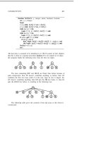
actually visited in the order A F E G D C B H I J K L M. Each connected
component leads to a tree, called the depth-first search tree. It is important
to note that this forest of depth-first search trees is simply another way of
drawing the graph; all vertices and edges of the graph are examined by the
algorithm.
Solid lines in the diagram indicate that the lower vertex was found by the
algorithm to be on the edge list of the upper vertex and had not been visited
at that time, so that a recursive call was made. Dotted lines correspond to
edges to vertices which had already been visited, so the if test in visit failed,
and the edge was not “followed” with a recursive call. These comments apply
to the time each edge is encountered; the if test in visit also guards
against following the edge the second time that it is encountered. For example,
once we’ve gone from A to F (on encountering F in A’s adjacency list), we
don’t want to go back from F to A (on encountering A in F’s adjacency list).
Similarly, dotted links are actually checked twice: even though we checked
that A was already visited while at G (on encountering A in G’s adjacency
list), we’ll check that G was already visited later on when we’re back at A (on
encountering G in A’s adjacency list).
A crucial property of these depth-first search trees for undirected graphs
is that the dotted links always go from a node to some ancestor in the tree
(another node in the same tree, that is higher up on the path to the root).
At any point during the execution of the algorithm, the vertices divide into
three classes: those for which visit has finished, those for which visit has only
partially finished, and those which haven’t been seen at all. By definition of
visit, we won’t encounter an edge pointing to any vertex in the first class,
and if we encounter an edge to a vertex in the third class, a recursive call
will be made (so the edge will be solid in the depth-first search tree). The
only vertices remaining are those in the second class, which are precisely the
vertices on the path from the current vertex to the root in the same tree, and
any edge to any of them will correspond to a dotted link in the depth-first

search tree.
The running time of dfs is clearly proportional to V + E for any graph.
We set each of the V val values (hence the V term), and we examine each
edge twice (hence the E term).
The same method can be applied to graphs represented with adjacency
matrices by using the following visit procedure:
384
CHAPTER 29
procedure integer);
var integer;
begin
:=now;
for to Vdo
if then
if then visit(t);
end
Traveling through an adjacency list translates to scanning through a row in
the adjacency matrix, looking for true values (which correspond to edges). As
before, any edge to a vertex which hasn’t been seen before is “followed” via
a recursive call. Now, the edges connected to each vertex are examined in a
different order, so we get a different depth-first search forest:
This underscores the point that the depth-first search forest is simply
another representation of the graph whose particular structure depends both
on the search algorithm and the internal representation used. The running
time of dfs when this visit procedure is used is proportional to since every
bit in the adjacency matrix is checked.
Now, testing if a graph has a cycle is a trivial modification of the above
program. A graph has a cycle if and only if a nonaero val entry is discovered
in visit. That is, if we encounter an edge pointing to a vertex that we’ve
already visited, then we have a cycle. Equivalently, all the dotted links in the

depth-first search trees belong to cycles.
Similarly, depth-first search finds the connected components of a graph.
Each nonrecursive call to visit corresponds to a different connected component.
An easy way to print out the connected components is to have visit print out
ELEMENTARY 385
the vertex being visited (say, by inserting just before exiting),
then print some indication that a new connected component is to start
just before the call to visit, in dfs (say, by inserting two statements).
This technique would produce the following output when dfs is used on the
adjacency list representation of our sample graph:
GDEFCBA
I H
KMLJ
Note that the adjacency matrix version of visit will compute the same con-
nected components (of course), but that the vertices will be printed out in a
different order.
Extensions to do more complicated processing on the connected com-
ponents are straightforward. For example, by simply inserting invaJ[now]=k
after vaJ[k]=now we get the “inverse”
of the array, whose nowth entry
is the index of the nowth vertex visited. (This is similar to the inverse heap
that we studied at the end of Chapter 11, though it serves a quite different
purpose.) Vertices in the same connected components are contiguous in this
array, the index of each new connected component given by the value of now
each time visit is called in dfs. These values could be stored, or used to mark
delimiters in (for example, the first entry in each connected component
could be made negative). The following table would be produced for our
example if the adjacency list version of dfs were modified in this way:
k name(k)
1

A
1
-1
2
B
7 6
3
C
6 5
4 D 5 7
5
E
3
4
6
F
2 3
7
G
4 2
8
H
8
-8
9
I
9
9
10
J

10
-10
11
K
11 11
12
L
12 12
13 M 13 13
With such techniques, a graph can be divided up into its connected
386
CHAPTER 29
ponents for later processing by more sophisticated algorithms.
Mazes
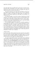
This systematic way of examining every vertex and edge of a graph has a
distinguished history: depth-first search was first stated formally hundreds
of years ago as a method for traversing mazes. For example, at left in the
diagram below is a popular maze, and at right is the graph constructed by
putting a vertex at each point where there is more than one path to take,
then connecting the vertices according to the paths:
This is significantly more complicated than early English garden mazes,
which were constructed as paths through tall hedges. In these mazes, all
walls were connected to the outer walls, so that gentlemen and ladies could
stroll in and clever ones could find their way out by simply keeping their
right hand on the wall (laboratory mice have reportedly learned this trick).
When independent inside walls can occur, it is necessary to resort to a more
sophisticated strategy to get around in a maze, which leads to depth-first
search.
To use depth-first search to get from one place to another in a maze, we
use visit, starting at the vertex on the graph corresponding to our starting

point. Each time visit “follows” an edge via a recursive call, we walk along
the corresponding path in the maze. The trick in getting around is that we
must walk back along the path that we used to enter each vertex when visit
finishes for that vertex. This puts us back at the vertex one step higher up
in the depth-first search tree, ready to follow its next edge.
The maze graph given above is an interesting “medium-sized” graph
which the reader might be amused to use as input for some of the algorithms in
later chapters. To fully capture the correspondence with the maze, a weighted
ELEMENTARY GRAPH ALGORITHMS 387
version of the graph should be used, with weights on edges corresponding to
distances (in the maze) between vertices.
Perspective
In the chapters that follow we’ll consider a variety of graph algorithms largely
aimed at determining connectivity properties of both undirected and directed
graphs. These algorithms are fundamental ones for processing graphs, but
are only an introduction to the subject of graph algorithms. Many interesting
and useful algorithms have been developed which are beyond the scope of
this book, and many interesting problems have been studied for which good
algorithms have not yet been found.
Some very efficient algorithms have been developed which are much too
complicated to present here. For example, it is possible to determine efficiently
whether or not a graph can be drawn on the plane without any intersecting
lines. This problem is called the planarity problem, and no efficient algorithm
for solving it was known until 1974, when R. E. developed an ingenious
(but quite intricate) algorithm for solving the problem in linear time, using
depth-first search.
Some graph problems which arise naturally and are easy to state seem
to be quite difficult, and no good algorithms are known to solve them. For
example, no efficient algorithm is known for finding the minimum-cost tour
which visits each vertex in a weighted graph. This problem, called the

traveling salesman problem, belongs to a large class of difficult problems that
we’ll discuss in more detail in Chapter 40. Most experts believe that no
efficient algorithms exist for these problems.
Other graph problems may well have efficient algorithms, though none has
been found. An example of this is the graph isomorphism problem: determine
whether two graphs could be made identical by renaming vertices. Efficient
algorithms are known for this problem for many special types of graphs, but
the general problem remains open.
In short, there is a wide spectrum of problems and algorithms for dealing
with graphs. We certainly can’t expect to solve every problem which comes
along, because even some problems which appear to be simple are still baffling
the experts. But many problems which are relatively easy to solve do arise
quite often, and the graph algorithms that we will study serve well in a great
variety of applications.