- Trang chủ >>
- Văn bản WTO >>
- WTO_Văn bản
MÔ HÌNH HÓA VÀ PHÂN TÍCH ĐỘNG HỌC CỦA HỆ THỐNG CẦU TRỤC 3D KHI THAY ĐỔI LỰC NÂNG HẠ VÀ KHỐI LƯỢNG TẢI TRỌNG
Bạn đang xem bản rút gọn của tài liệu. Xem và tải ngay bản đầy đủ của tài liệu tại đây (334.82 KB, 8 trang )
<span class='text_page_counter'>(1)</span><div class='page_container' data-page=1>
<b>DYNAMIC MODELING AND ANALYSIS OF A THREE – DIMENTIONAL </b>
<b>OVERHEAD CRANE SYSTEM WITH THE VARIATION </b>
<b>OF LOAD MASS AND HOISTING/LOWERING FORCE </b>
<b>Nguyen Trung Thanh1*, Nguyen Thanh Tien2, Tran Ngoc Quy 3, Nguyen Thi Thu Hang1 </b>
<i>1</i>
<i>Hung Yen University of Technology and Education, 2Minitary Technical Academy </i>
<i>3</i>
<i>Science and Technology Institute of Military </i>
ABSTRACT
Cranes are commonly used in the industry, in the military to move heavy loads, or assembly of
large structures. Three basic movements of the crane is moving vertically, horizontally and lifting
loads. However, the vibration of the load during move affects the safety and operational efficiency
of the system. The velocity escalation to enhance performance as the vibration is caused by losing
of time and counterproductive. This paper proposes solutions to improve the efficiency of the
crane in conditions of appropriate parameters. A dynamic model of the overhead crane system is
also developed in three-dimensional space based on Euler- Lagrange method, including the
description of the movement of the load in the vertical, horizontal and lifting direction. Effects of
parameters variation as load mass, hoisting/ lowering force on the response of the system on the
<b>time domain and frequency domain are discussed through simulation results. The article also </b>
suggestes the parameter range to work effectively. Finally, some conclusions are presented.
<i><b>Keywords: Dynamical models; 3D crane; Euler- Lagrange method; time domain and frequency </b></i>
<i>domain; power spectral density, effective parameter range</i>
INTRODUCTION*
Overhead crane systems in three-dimensional
(3-D crane) often used to transport heavy
loads in factories and habors.... During speed
acceleration or reduction always cause
unwanted load swing at the destination
location. Disturbances such as friction, wind
and rain also reduces performance overhead
cranes, it adversely impacts on the crane
performance. These problems reduce the
efficiency of work. In some cases, they cause
damages to the load or become unsafe.
Therefore, the divelopement and analysis of
dynamic models with the change of crane
parameters is necessary to promote the
working efficiency of the crane.
The mathematical description and nonlinear
control as the crane was studied from the
early age [8,10,11,13,14]. The development
of a nonlinear dynamical models and methods
for crane control 2-D, 3-D have been written
in many reports [1,6-8]. Most of the reports
focuse on the issue of handling to minimize
*
<i>Tel: 0982 829684</i>
</div>
<span class='text_page_counter'>(2)</span><div class='page_container' data-page=2>
MODELING OF A THREE
DIMENTIO-NAL OVERHEAD CRANE
Figure 1 describes the coordinate system of a
<i>3-D crane and its load. XYZ is set as a fixed </i>
<i>coordinate system and XcYcZc</i> as trolleys. The
axis of the trolley coordinate system are
paralleled respectively fixed coordinate
<i>system. The girder moves along the Xc</i> axis.
<i>The trolley moves along the Yc</i> axis.
Coordinates of the trolley and load are shown
as the figure. is the swing angle of the load
in a space and is subcategorized into two
components:
<i><sub>x</sub></i> and <i><sub>y</sub>. l is the rope length </i>from the trolley to the load.
<i><b>Figure 1. The description of the 3-D crane </b></i>
<i>The position of load (xp, yp, zp</i>) in fixed
coordinate can be performed:
<i>y</i>
<i>x</i>
<i>p</i>
<i>y</i>
<i>p</i>
<i>y</i>
<i>x</i>
<i>p</i>
<i>l</i>
<i>z</i>
<i>l</i>
<i>y</i>
<i>y</i>
<i>l</i>
<i>x</i>
<i>x</i>
cos
cos
;
sin
;
cos
sin
(1)
This study refers to three simultaneous
movement of girder, trolley and load.
Therefore, the parameters x, y, l,
<i><sub>x</sub></i> and <i><sub>y</sub></i> isdefined in the general coordinates to describe
motion of overhead crane.
The motion of 3-D overhead crane is based on
Lagrange’s equation. Here the load is assumed
as a point mass located at the center. The mass
and the springiness of the rope are ignored. T is
called the kinetic energy of cranes including the
girder, the trolley and the load; P is called the
potential energy of the crane.
<i>(2) </i>
where Mx is a traveling component of the
crane system mass, My is a traversing
component and Ml is a hoisting component.
<i>m, g and vp</i> are the load mass, the gravity and
the load velocity, respectively.
<i>y</i>
<i>l</i>
<i>l</i>
<i>x</i>
<i>l</i>
<i>l</i>
<i>l</i>
<i>l</i>
<i>l</i>
<i>l</i>
<i>y</i>
<i>x</i>
<i>z</i>
<i>y</i>
<i>x</i>
<i>v</i>
<i>y</i>
<i>y</i>
<i>y</i>
<i>y</i>
<i>y</i>
<i>x</i>
<i>x</i>
<i>y</i>
<i>x</i>
<i>y</i>
<i>x</i>
<i>y</i>
<i>x</i>
<i>y</i>
<i>p</i>
<i>p</i>
<i>p</i>
<i>p</i>
)
cos
(sin
2
)
sin
sin
cos
cos
cos
(sin
2
cos2 2 2 2
2
2
2
2
2
2
2
2
<i>(4) </i>
The Lagrange function is defined as:
The dissipation function (mainly due to
friction) is defined as follows:
)
(
2
1 2 2 2
<i>l</i>
<i>D</i>
<i>y</i>
<i>D</i>
<i>x</i>
<i>Dx</i> <i>y</i> <i>l</i>
(6)
<i>where Dx, Dy và Dl denote the viscous </i>
<i>damping coefficients according to the x, y and </i>
<i>l motion. </i>
The general Lagrange equations is written:
)
5
1
(
)
(
<i>i</i>
<i>F</i>
<i>q</i>
<i>q</i>
<i>P</i>
<i>q</i>
<i>T</i>
<i>q</i>
<i>T</i>
<i>dt</i>
<i>d</i>
<i>i</i>
<i>q</i>
<i>i</i>
<i>i</i>
<i>i</i>
<i>i</i>
(7)
<i>where Fqi</i> is the corresponding generalized
<i>force ith, which belongs to the generalized </i>
coordinate system. The equations of motion
of the crane system are defined by inserting L
and in Lagrange equations with the
<i>generalized coordinate system x, y, l, </i>
<i><sub>x</sub>,</i><i><sub>y</sub></i>:<i>x</i>
<i>y</i>
<i>y</i>
<i>x</i>
<i>y</i>
<i>x</i>
<i>y</i>
<i>x</i>
<i>x</i>
<i>y</i>
<i>x</i>
<i>y</i>
<i>y</i>
<i>x</i>
<i>x</i>
<i>y</i>
<i>x</i>
<i>x</i>
<i>y</i>
<i>x</i>
<i>y</i>
<i>y</i>
<i>x</i>
<i>x</i>
<i>y</i>
<i>x</i>
<i>x</i>
<i>f</i>
<i>ml</i>
<i>ml</i>
<i>ml</i>
<i>l</i>
<i>m</i>
<i>l</i>
<i>m</i>
<i>x</i>
<i>D</i>
<i>l</i>
<i>m</i>
<i>ml</i>
<i>ml</i>
<i>x</i>
<i>m</i>
<i>M</i>
2
2
cos
sin
sin
cos
2
cos
sin
sin
sin
2
cos
cos
2
cos
sin
sin
sin
cos
cos
)
(
(8)
<i>y</i>
<i>y</i>
<i>y</i>
<i>y</i>
<i>y</i>
<i>y</i>
<i>y</i>
<i>y</i>
<i>y</i>
<i>y</i>
<i>f</i>
<i>ml</i>
<i>l</i>
<i>m</i>
<i>y</i>
<i>D</i>
<i>l</i>
<i>m</i>
<i>ml</i>
<i>y</i>
<i>m</i>
<i>M</i>
2
sin
cos
2
sin
cos
)
(
(9)
x
y
X
Z
Y
Xc
Yc
(0,0,0)
(x,y,0)
y
x
(xp,yp,zp)
</div>
<span class='text_page_counter'>(3)</span><div class='page_container' data-page=3>
<i>l</i>
<i>y</i>
<i>x</i>
<i>y</i>
<i>x</i>
<i>y</i>
<i>l</i>
<i>y</i>
<i>y</i>
<i>x</i>
<i>l</i>
<i>f</i>
<i>mg</i>
<i>ml</i>
<i>ml</i>
<i>l</i>
<i>D</i>
<i>y</i>
<i>m</i>
<i>x</i>
<i>m</i>
<i>l</i>
<i>m</i>
<i>M</i>
cos
cos
cos
sin
cos
sin
)
(
2
2
2
(10)
0
cos
sin
cos
sin
2
cos
2
cos
cos
cos
2
2
2
2
<i>y</i>
<i>x</i>
<i>y</i>
<i>x</i>
<i>y</i>
<i>y</i>
<i>x</i>
<i>y</i>
<i>y</i>
<i>x</i>
<i>x</i>
<i>y</i>
<i>mgl</i>
<i>ml</i>
<i>l</i>
<i>ml</i>
<i>x</i>
<i>ml</i>
<i>ml</i>
(11)
0
sin
cos
sin
cos
2
sin
sin
cos
2
2
2
<i>y</i>
<i>x</i>
<i>x</i>
<i>y</i>
<i>y</i>
<i>y</i>
<i>y</i>
<i>x</i>
<i>y</i>
<i>y</i>
<i>mgl</i>
<i>ml</i>
<i>l</i>
<i>ml</i>
<i>x</i>
<i>ml</i>
<i>y</i>
<i>ml</i>
<i>ml</i>
(12)
<i>where fx, fy, fl</i> are the driving force of the
<i>girders, the trolley and the load for the x, y, l </i>
motions, respectively.
The dynamic model of crane is equivalent to
the dynamic model of robot having three soft
bindings. The dynamic model (8) - (12) can
be performed in the form of the matrix vector,
as follows:
<i>F</i>
<i>q</i>
<i>G</i>
<i>q</i>
<i>q</i>
<i>q</i>
<i>C</i>
<i>q</i>
<i>D</i>
<i>q</i>
<i>q</i>
<i>M</i>( ) (, ) ( ) (13)
<i>where q is the state vector, F is the driving </i>
<i>force vector, G(q) is gravitational vector and </i>
<i>D is dissipation matrix because of the friction, </i>
respectively:
<i>T</i>
<i>y</i>
<i>x</i>
<i>l</i>
<i>y</i>
<i>x</i>
<i>q</i>
[
,
,
,
,
]
<i>T</i>
<i>l</i>
<i>y</i>
<i>x</i> <i>f</i> <i>f</i>
<i>f</i>
<i>F</i> [ , , , 0 , 0]
<i>T</i>
<i>y</i>
<i>x</i>
<i>y</i>
<i>x</i>
<i>y</i>
<i>x</i>
<i>mgl</i>
<i>mgl</i>
<i>mg</i>
<i>q</i>
<i>G</i>
)
sin
cos
,
cos
sin
,
cos
cos
,
0
,
0
(
)
(
)
0
,
0
,
,
,
(<i>D<sub>x</sub></i> <i>D<sub>y</sub></i> <i>D<sub>l</sub></i>
<i>diag</i>
<i>D</i>
<i>The symmetric mass matrix M(q) </i><i> R(5 x 5)</i> is
denoted:
55
52
51
44
41
33
32
31
25
23
22
15
14
13
11
0
0
0
0
0
0
0
0
0
0
)
(
<i>m</i>
<i>m</i>
<i>m</i>
<i>m</i>
<i>m</i>
<i>m</i>
<i>m</i>
<i>m</i>
<i>m</i>
<i>m</i>
<i>m</i>
<i>m</i>
<i>m</i>
<i>m</i>
<i>m</i>
<i>q</i>
<i>M</i>
;
cos
;
cos
cos
;
;
sin
;
cos
sin
;
cos
;
sin
;
;
sin
sin
;
cos
cos
;
cos
sin
;
2
2
44
41
33
32
31
25
23
22
15
14
13
11
<i>y</i>
<i>y</i>
<i>x</i>
<i>l</i>
<i>y</i>
<i>y</i>
<i>x</i>
<i>y</i>
<i>y</i>
<i>y</i>
<i>y</i>
<i>x</i>
<i>y</i>
<i>x</i>
<i>y</i>
<i>x</i>
<i>x</i>
<i>ml</i>
<i>m</i>
<i>ml</i>
<i>m</i>
<i>m</i>
<i>M</i>
<i>m</i>
<i>m</i>
<i>m</i>
<i>m</i>
<i>m</i>
<i>ml</i>
<i>m</i>
<i>m</i>
<i>m</i>
<i>m</i>
<i>M</i>
<i>m</i>
<i>ml</i>
<i>m</i>
<i>ml</i>
<i>m</i>
<i>m</i>
<i>m</i>
<i>m</i>
<i>M</i>
<i>m</i>
2
55
52
51 <i>ml</i>sin sin ;<i>m</i> <i>ml</i>cos ;<i>m</i> <i>ml</i>
<i>m</i> <i><sub>x</sub></i> <i><sub>y</sub></i> <i><sub>y</sub></i>
<i>M(q) is positive definite when l > 0 and </i>
2
/
<i>y</i> <i>. C( q ,q) </i><i> R</i>
5x5
is the matrix of
centrifugal force and Coriolis.
55
54
53
45
44
43
35
34
25
23
15
14
13
0
0
0
0
0
0
0
0
0
0
0
0
)
,
(
<i>c</i>
<i>c</i>
<i>c</i>
<i>c</i>
<i>c</i>
<i>c</i>
<i>c</i>
<i>c</i>
<i>c</i>
<i>c</i>
<i>c</i>
<i>c</i>
<i>c</i>
<i>q</i>
<i>q</i>
<i>C </i>
;
sin
cos
;
cos
;
cos
sin
sin
cos
sin
sin
;
sin
cos
cos
sin
cos
cos
;
sin
sin
cos
cos
25
23
15
14
13
<i>y</i>
<i>y</i>
<i>y</i>
<i>y</i>
<i>y</i>
<i>y</i>
<i>y</i>
<i>x</i>
<i>x</i>
<i>y</i>
<i>x</i>
<i>y</i>
<i>x</i>
<i>y</i>
<i>y</i>
<i>x</i>
<i>x</i>
<i>y</i>
<i>x</i>
<i>y</i>
<i>x</i>
<i>y</i>
<i>y</i>
<i>x</i>
<i>x</i>
<i>y</i>
<i>x</i>
<i>ml</i>
<i>l</i>
<i>m</i>
<i>c</i>
<i>m</i>
<i>c</i>
<i>ml</i>
<i>ml</i>
<i>l</i>
<i>m</i>
<i>c</i>
<i>ml</i>
<i>ml</i>
<i>l</i>
<i>m</i>
<i>c</i>
<i>m</i>
<i>m</i>
<i>c</i>
;
;
sin
cos
;
;
cos
sin
;
cos
sin
cos
;
cos
;
;
cos
55
2
54
53
2
45
2
2
44
2
43
35
2
34
<i>l</i>
<i>ml</i>
<i>c</i>
<i>ml</i>
<i>c</i>
<i>ml</i>
<i>c</i>
<i>ml</i>
<i>c</i>
<i>ml</i>
<i>l</i>
<i>ml</i>
<i>c</i>
<i>ml</i>
<i>c</i>
<i>ml</i>
<i>c</i>
<i>ml</i>
<i>c</i>
<i>x</i>
<i>y</i>
<i>y</i>
<i>y</i>
<i>x</i>
<i>y</i>
<i>y</i>
<i>y</i>
<i>y</i>
<i>y</i>
<i>y</i>
<i>x</i>
<i>y</i>
<i>y</i>
<i>x</i>
<i>y</i>
SIMULATION OF CRANE SYSTEM
RESPONSE WITH VARIABLE PARAME-TERS
In this section, the dynamic of 3-D crane (13)
will be analyzed in the time domain and
frequency domain. The values of the nominal
parameters are determined by crane models in
the laboratory:
0
;
8
;
30
;
60
;
85
.
0
;
/
50
;
85
.
2
;
/
20
;
85
.
5
;
/
30
;
85
.
12
<i>l</i>
<i>N</i>
<i>f</i>
<i>N</i>
<i>f</i>
<i>N</i>
<i>f</i>
<i>kg</i>
<i>m</i>
<i>m</i>
<i>Ns</i>
<i>D</i>
<i>kg</i>
<i>M</i>
<i>m</i>
<i>Ns</i>
<i>D</i>
<i>kg</i>
<i>M</i>
<i>m</i>
<i>Ns</i>
<i>D</i>
<i>kg</i>
<i>M</i>
<i>l</i>
<i>y</i>
<i>x</i>
<i>l</i>
<i>l</i>
<i>y</i>
<i>y</i>
<i>x</i>
<i>x</i>
The gravity acceleration is 2
/
8
.
9 <i>m</i> <i>s</i>
<i>g</i> .
Simulation time is 10s, the sampling time is
1ms. The position and swing angle responses
of the system and the power spectral density
are analyzed and evaluated.
</div>
<span class='text_page_counter'>(4)</span><div class='page_container' data-page=4>
<b>The system response with different loads </b>
To observe the affects of the payload on the
system dynamic, various payloads are
simulated. The results showed most clearly
when the mass of load changes from 0,85kg
to 5,50kg. Figure 3 shows the position
responses in the x, y, z axis. There are no
large oscillation in the position response .
Table 1 synthesizes the relation between the
mass of load and the trolley positions.
Respectively, figures 4 and 5 indicated
responses of swing angle in the x and y
directions when the mass of the load is
changed. This relationship has also been
summarized as in the Table 1.
0 1 2 3 4 5 6 7 8 9
0
5
10
15
time(s)
p
o
s
it
io
n
x
(m
)
m=0.85kg
m=2.85kg
m=4.85kg
<i><b>Figure 3. Position response in the x directions </b></i>
<i>with variation of payload</i>
0 1 2 3 4 5 6 7 8 9 10
0
5
10
15
time(s)
p
o
s
it
io
n
(y
)
m=0.85kg
m=2.85kg
m=4.85kg
<i><b>Figure 4. Position response in the y directions </b></i>
<i>with variation of payload</i>
0 1 2 3 4 5 6 7 8 9 10
0
1
2
3
4
5
time(s)
p
o
s
it
io
n
l
(m
)
m=0.85kg
m=2.85kg
m=4.85kg
<i><b>Figure 5. Position response in the z directions </b></i>
<i>with variation of payload</i>
0 1 2 3 4 5 6 7 8 9 10
-0.8
-0.6
-0.4
-0.2
0
0.2
0.4
0.6
time(s)
th
e
ta
(x
)
m=0.85kg
m=2.85kg
m=4.85kg
<i><b>Figure 6. Swing angle </b></i><i>x with variation of payload </i>
0 1 2 3 4 5 6 7 8 9 10
-0.6
-0.4
-0.2
0
0.2
time(s)
th
e
ta
(y
)
m=0.85kg
m=2.85kg
m=4.85kg
<i><b>Figure 7. Swing angle </b></i><i>y with variation of payload </i>
0 0.05 0.1 0.15 0.2 0.25 0.3 0.35 0.4
-60
-40
-20
0
20
Frequency (Hz)
M
a
g
n
it
u
d
e
(
d
B
)
m=0.85kg
m=2.85kg
m=4.85kg
<i><b>Figure 8. Power spectral density of </b></i><i>x </i>
<i>with variation of payload </i>
0 0.05 0.1 0.15 0.2 0.25 0.3 0.35 0.4
-60
-40
-20
0
20
Frequency (Hz)
M
a
g
n
it
u
d
e
(
d
B
)
Frequency domain
m=0.85kg
m=2.85kg
m=4.85kg
<i><b>Figure 9. Power spectral density </b></i>
<i>of </i><i>y with variation of payload</i>
<i><b>Table 1. The relation between</b>variation of payloadwith trolley position and swing angles </i>
<b>Payload (kg) </b> <b>Trolley position (m) (average) </b> <b>Swing angles (max-min) </b>
<b>x direction </b> <b>y direction </b> <b>z direction </b> <b>x (rad) </b> <b>y (rad) </b>
m=0.85 5.863 4.533 0.1351 ±0.6626 ±0.5112
m=1.50 5.797 4.456 0.5295 ±0.5336 ±0.4196
m=2.85 5.670 4.310 1.3700 ±0.4076 ±0.3150
m=3.50 5.611 4.243 1.7620 ±0.3724 ±0.2839
m=4.85 5.491 4.108 2.3270 ±0.3219 ±0.2383
</div>
<span class='text_page_counter'>(5)</span><div class='page_container' data-page=5>
The findings show that if the mass of load is
increased, the swing angle will decrease,
vibration frequency will also decrease,
oscillation period will be shorter. Figure 7 and
Figure 8 shows the power spectral density
corresponding to the swing angle in the x
direction and the y direction. It proves that the
resonance with oscillation frequency
increases when the load increases. Thus, this
study shows that in order to reduce the
vibrations of the system, we can limit the
range of the load mass. Accordingly, this
range is called “effective parameter range„.
Even then, if the system is not yet equipped
with modern controllers, high performance
with “effective parameter range„ is
maintained. In this case, when the load mass
is within 4kg to 5kg. Swing angle and also
frequency reduces, the settling time is less
than 3 seconds.
<b>The system response with different hoisting force </b>
To observe more clearly the effects of the
system parameters to the vibration of the load,
especially hoisting force, here we consider fl
= [-20N, 20N]. Girder force, trolley force and
other parameters are constant.
0 1 2 3 4 5 6 7 8 9 10
-1.5
-1
-0.5
0
0.5
1
1.5
time (s)
th
e
ta
(x
)
(r
a
d
)
fl = - 15N
fl = - 10N
fl = 10N
fl = 15N
<i><b>Figure 10. Swing angle </b></i><i>x with variation </i>
<i>of hoisting force</i>
0 1 2 3 4 5 6 7 8 9 10
-1.5
-1
-0.5
0
0.5
1
1.5
time(s)
th
e
ta
(y
)
(r
a
d
)
fl = - 15N
fl = - 10N
fl= 10 N
fl = 15N
<i><b>Figure 11. Swing angle </b></i><i>y with variation </i>
<i>of hoisting force </i>
0 0.005 0.01 0.015 0.02 0.025 0.03 0.035 0.04 0.045 0.05
-20
0
20
40
60
Frequency (Hz)
M
a
g
n
it
u
d
e
(
d
B
)
Frequency domain
fl = - 15N
fl = - 10N
fl = 10N
fl = 15N
<i><b>Figure 12. Power spectral densitys of swing </b></i>
<i>angle </i><i>x with variation of hoisting force </i>
0 0.005 0.01 0.015 0.02 0.025 0.03 0.035 0.04 0.045 0.05
-20
0
20
40
60
Frequency (Hz)
M
a
g
n
it
u
d
e
(
d
B
)
Frequency domain
fl = - 15N
fl = - 10N
fl = 10N
fl = 15N
<i><b>Figure 13. The power spectral density of swing </b></i>
<i>angle </i><i>x with variation of hoisting force </i>
<i><b>Table 2. Relation between hoisting force </b></i>
<i>with swing angles </i>
<b>Hoisting force </b>
<b>(N) </b>
<b>Swing angle (max-min) </b>
<b>x (rad) </b> <b>y (rad) </b>
fl = -15 ±1.271 ±1.251
fl = -10 ±0.7208 ±0.5383
</div>
<span class='text_page_counter'>(6)</span><div class='page_container' data-page=6>
is less than 1 second, the overshoot is about
12%, oscillation frequency is also smaller. The
results confirmed that it is not neccessary to
design a new controller if the hoisting force is
varied within the “effective parameter range„.
CONCLUSION
This study presents the development of a
dynamics model of a 3-D overhead crane base
on the Euler-Lagrange approach. The model
was simulated with bang – bang force input.
The trolley position and the swing angle
response have been described and analyzed in
the time domain and frequency domain. The
affection of mass load, hoisting force to the
dynamic characteristic of the system are also
analyzed also discussed. These results are
very useful and important to develop
effective control methods and control
algorithms for the system 3-D crane with
different loads and driving forces.
REFERENCES
1. Ahmad, M.A., Mohamed, Z. and Hambali, N.
(2008), “Dynamic Modelling of a Two-link
Flexible Manipulator System Incorporating
<i>Payload”, 3rd IEEE Conference on Industrial </i>
<i>Electronics and Applications, pp. 96-101.</i>
2. B. D’Andrea-Novel and J. M. Coron,
“Stabilization of an overhead crane with a variable
<i>length flexible cable,” Computational and Applied </i>
<i>Mathematics, vol. 21, no. 1, pp. 101-134, 2002</i>.
3. Blajer, W. and Kolodziejczyk, K. (2007),
“Motion Planning and Control of Gantry Cranes in
<i>Cluttered Work Environment”, IET Control </i>
<i>Theory Applications, Vol. 1, No. 5, pp. </i>
1370-1379.
4. Chang, C.Y. and Chiang, K.H. (2008), “Fuzzy
Projection Control Law and its Application to the
<i>Overhead Crane”, Journal of Mechatronics, Vol. </i>
18, pp. 607-615.
5. Fang, Y., Dixon, W.E., Dawson, D.M. and
Zergeroglu, E. (2003), “Nonlinear Coupling
Control Laws for an Underactuated Overhead
Crane System”, <i>IEEE/ASME </i> <i>Trans. </i> <i>On </i>
<i>Mechatronics, Vol. 8, No. 3, pp. 418-423. </i>
6. Ismail, et al. (2009), “Nonlinear Dynamic
Modelling and Analysis of a 3-D Overhead Gantry
<i>Crane System with Payload Variation”, Third </i>
<i>UKSim European Symposium on Computer </i>
<i>Modeling and Simulation, pp. 350-354.</i>
7. J. W. Auernig and H. Troger, “Time optimal
control of overhead cranes with hoisting of the
<i>load,” Automatica, vol. 23, no. 4, pp. 437-447, </i>
1987.
8. Lee, H.H. (1998), “Modeling and Control of a
<i>Three-Dimensional Overhead Crane”, Journal of </i>
<i>Dynamics Systems, Measurement, and Control, </i>
Vol. 120, pp. 471-476.
9. Piazzi, A. and Visioli, A. (2002), “Optimal
Dynamic-inversion-based Control of an Overhead
<i>Crane”, IEE Proc. Control Theory Application, </i>
Vol. 149, No. 5, pp. 405-411.
10. Spong, M.W. (1997), “Underactuated
Mechanical Systems, Control Problems in
Robotics and Automation”, London:
Springer-Verlag.
11. Spong, M.W., Hutchinson, S. and Vidyasagar,
M. (2006), “Robot Modeling and Control”, New
Jersey: John Wiley.
12. Y. B. Kim, et al., “An anti-sway control
system design based on simultaneous optimization
<i>design approach,” Journal of Ocean Engineering </i>
<i>and Technology (in Korean), vol. 19, no. 3, pp. </i>
66-73, 2005.
13. Y. Sakawa and Y. Shindo, “Optimal control of
<i>container cranes,” Automatica, vol. 18, no. 3, pp. </i>
257-266, 1982.
14. Y. Sakawa and H. Sano, “Nonlinear model and
linear robust control of overhead traveling cranes,”
<i>Nonlinear Analysis, Theory, Methods & </i>
</div>
<span class='text_page_counter'>(7)</span><div class='page_container' data-page=7>
T M T T
<b>MƠ HÌNH HĨA VÀ PHÂN TÍCH ĐỘNG HỌC CỦA HỆ THỐNG CẦU TRỤC 3D </b>
<b>KHI THAY ĐỔI LỰC NÂNG HẠ VÀ KHỐI LƯỢNG TẢI TRỌNG </b>
<b>Nguyễn Trung Thành1*<sub>, Nguyễn Thanh Tiên</sub>2<sub>, </sub></b>
<b>Trần Ngọc Quý 3<sub>,Nguyễn Thị Thu Hằng</sub>1 </b>
<i>1<sub>Trường Đại học Sư phạm Kỹ thuật Hưng Yên, </sub></i>2<i><sub>Học viện Kỹ thuật Quân sự </sub></i>
<i>3<sub>Viện Khoa học và Công nghệ Quân sự</sub></i>
Cầu trục được sử dụng rất phổ biến trong công nghiệp, trong quân sự để di chuyển những trọng tải
nặng, hoặc lắp ghép những cấu kiện lớn. Ba chuyển động cơ bản của cầu trục là hành trình học,
hành trình ngang và nâng hạ tải trọng. Sự rung lắc của tải trọng khi di chuyển đe dọa đến vấn đề an
toàn và ảnh hưởng đến hiệu quả làm việc. Tăng tốc độ làm việc nhằm nâng cao hiệu suất càng gây
ra sự rung lắc làm hao tổn thời gian, dẫn đến không đạt kết quả mong muốn. Bài viết này phân tích
và đề xuất giải pháp nâng cao hiệu quả khi cho cầu trục làm việc trong điều kiện tham số thích
hợp. Bài viết đồng thời mô tả mô hình động lực học của hệ thống cầu trục trong không gian ba
chiều dựa vào phương pháp Euler- Lagrange, gồm mô tả những chuyển động của tải trọng theo
hướng dọc, ngang và nâng hạ. Những ảnh hưởng của sự thay đổi khối lượng tải trọng và lực kéo
nâng hạ đến đáp ứng hệ thống trên miền thời gian và miền tần số được phân tích qua kết quả mô
phỏng. Bài báo cũng đề xuất vùng tham số làm việc hiệu quả. Cuối cùng là một số kết luận.
<i><b>T h a: Mô hình động học; cầu trục 3-D; phương pháp Euler- Lagrange; miền thời gian và </b></i>
<i>miền tần số; mật độ phổ công suất, vùng tham số hiệu quả </i>
*
</div>
<span class='text_page_counter'>(8)</span><div class='page_container' data-page=8></div>
<!--links-->