Microstrip bộ lọc cho các ứng dụng lò vi sóng RF (P3)
Bạn đang xem bản rút gọn của tài liệu. Xem và tải ngay bản đầy đủ của tài liệu tại đây (699.63 KB, 48 trang )
CHAPTER 3
Basic Concepts and
Theories of Filters
This chapter describes basic concepts and theories that form the foundation for de-
sign of general RF/microwave filters, including microstrip filters. The topics will
cover filter transfer functions, lowpass prototype filters and elements, frequency
and element transformations, immittance inverters, Richards’ transformation, and
Kuroda identities for distributed elements. Dissipation and unloaded quality factor
of filter elements will also be discussed.
3.1 TRANSFER FUNCTIONS
3.1.1 General Definitions
The transfer function of a two-port filter network is a mathematical description of
network response characteristics, namely, a mathematical expression of S
21
. On
many occasions, an amplitude-squared transfer function for a lossless passive filter
network is defined as
|S
21
( j⍀)|
2
= (3.1)
where
is a ripple constant, F
n
(⍀) represents a filtering or characteristic function,
and ⍀ is a frequency variable. For our discussion here, it is convenient to let ⍀ rep-
resent a radian frequency variable of a lowpass prototype filter that has a cutoff fre-
quency at ⍀ = ⍀
c
for ⍀
c
= 1 (rad/s). Frequency transformations to the usual radian
frequency for practical lowpass, highpass, bandpass, and bandstop filters will be
discussed later on.
1
ᎏᎏ
1 +
2
F
n
2
(⍀)
29
Microstrip Filters for RF/Microwave Applications. Jia-Sheng Hong, M. J. Lancaster
Copyright © 2001 John Wiley & Sons, Inc.
ISBNs: 0-471-38877-7 (Hardback); 0-471-22161-9 (Electronic)
For linear, time-invariant networks, the transfer function may be defined as a ra-
tional function, that is
S
21
(p) = (3.2)
where N(p) and D(p) are polynomials in a complex frequency variable p =
+ j⍀.
For a lossless passive network, the neper frequency
= 0 and p = j⍀. To find a real-
izable rational transfer function that produces response characteristics approximat-
ing the required response is the so-called approximation problem, and in many
cases, the rational transfer function of (3.2) can be constructed from the amplitude-
squared transfer function of (3.1) [1–2].
For a given transfer function of (3.1), the insertion loss response of the filter, fol-
lowing the conventional definition in (2.9), can be computed by
L
A
(⍀) = 10 log dB (3.3)
Since |S
11
|
2
+ |S
21
|
2
= 1 for a lossless, passive two-port network, the return loss re-
sponse of the filter can be found using (2.9):
L
R
(⍀) = 10 log[1 – |S
21
( j⍀)|
2
] dB (3.4)
If a rational transfer function is available, the phase response of the filter can be
found as
21
= Arg S
21
( j⍀) (3.5)
Then the group delay response of this network can be calculated by
d
(⍀) = seconds (3.6)
where
21
(⍀) is in radians and ⍀ is in radians per second.
3.1.2 The Poles and Zeros on the Complex Plane
The (
, ⍀) plane, where a rational transfer function is defined, is called the complex
plane or the p-plane. The horizontal axis of this plane is called the real or
-axis,
and the vertical axis is called the imaginary or j⍀-axis. The values of p at which the
function becomes zero are the zeros of the function, and the values of p at which the
function becomes infinite are the singularities (usually the poles) of the function.
Therefore, the zeros of S
21
(p) are the roots of the numerator N(p) and the poles of
S
21
(p) are the roots of denominator D(p).
These poles will be the natural frequencies of the filter whose response is de-
d
21
(⍀)
ᎏ
–d⍀
1
ᎏ
|S
21
( j⍀)|
2
N(p)
ᎏ
D(p)
30
BASIC CONCEPTS AND THEORIES OF FILTERS
scribed by S
21
(p). For the filter to be stable, these natural frequencies must lie in the
left half of the p-plane, or on the imaginary axis. If this were not so, the oscillations
would be of exponentially increasing magnitude with respect to time, a condition
that is impossible in a passive network. Hence, D(p) is a Hurwitz polynomial [3];
i.e., its roots (or zeros) are in the inside of the left half-plane, or on the j⍀-axis,
whereas the roots (or zeros) of N(p) may occur anywhere on the entire complex
plane. The zeros of N(p) are called finite-frequency transmission zeros of the filter.
The poles and zeros of a rational transfer function may be depicted on the p-
plane. We will see in the following that different types of transfer functions will be
distinguished from their pole-zero patterns of the diagram.
3.1.3 Butterworth (Maximally Flat) Response
The amplitude-squared transfer function for Butterworth filters that have an inser-
tion loss L
Ar
= 3.01 dB at the cutoff frequency ⍀
c
= 1 is given by
|S
21
( j⍀)|
2
= (3.7)
where n is the degree or the order of filter, which corresponds to the number of re-
active elements required in the lowpass prototype filter. This type of response is
also referred to as maximally flat because its amplitude-squared transfer function
defined in (3.7) has the maximum number of (2n – 1) zero derivatives at ⍀ = 0.
Therefore, the maximally flat approximation to the ideal lowpass filter in the pass-
band is best at ⍀ = 0, but deteriorates as ⍀ approaches the cutoff frequency ⍀
c
. Fig-
ure 3.1 shows a typical maximally flat response.
1
ᎏ
1 + ⍀
2n
3.1 TRANSFER FUNCTIONS
31
FIGURE 3.1 Butterworth (maximally flat) lowpass response.
A rational transfer function constructed from (3.7) is [1–2]
S
21
(p) = (3.8)
with
p
i
= j exp
΄΅
There is no finite-frequency transmission zero [all the zeros of S
21
(p) are at infini-
ty], and the poles p
i
lie on the unit circle in the left half-plane at equal angular spac-
ings, since |p
i
| = 1 and Arg p
i
= (2i – 1)
/2n. This is illustrated in Figure 3.2.
3.1.4 Chebyshev Response
The Chebyshev response that exhibits the equal-ripple passband and maximally flat
stopband is depicted in Figure 3.3. The amplitude-squared transfer function that de-
scribes this type of response is
|S
21
( j⍀)|
2
= (3.9)
where the ripple constant
is related to a given passband ripple L
Ar
in dB by
=
Ί
1
0
–
1
(3.10)
L
Ar
ᎏ
10
1
ᎏᎏ
1 +
2
T
n
2
(⍀)
(2i – 1)
ᎏ
2n
1
ᎏᎏ
n
⌸
i=1
(p – p
i
)
32
BASIC CONCEPTS AND THEORIES OF FILTERS
FIGURE 3.2 Pole distribution for Butterworth (maximally flat) response.
T
n
(⍀) is a Chebyshev function of the first kind of order n, which is defined as
T
n
(⍀) =
Ά
(3.11)
Hence, the filters realized from (3.9) are commonly known as Chebyshev filters.
Rhodes [2] has derived a general formula of the rational transfer function from
(3.9) for the Chebyshev filter, that is
S
21
(p) = (3.12)
with
p
i
= j cos
΄
sin
–1
j
+
΅
= sinh
sinh
–1
Similar to the maximally flat case, all the transmission zeros of S
21
(p) are located at
infinity. Therefore, the Butterworth and Chebyshev filters dealt with so far are
sometimes referred to as all-pole filters. However, the pole locations for the Cheby-
shev case are different, and lie on an ellipse in the left half-plane. The major axis of
the ellipse is on the j⍀-axis and its size is
͙
1
ෆ
+
ෆ
ෆ
2
ෆ
; the minor axis is on the
-axis
and is of size
. The pole distribution is shown, for n = 5, in Figure 3.4.
1
ᎏ
1
ᎏ
n
(2i – 1)
ᎏ
2n
n
⌸
i=1
[
2
+ sin
2
(i
/n)]
1/2
ᎏᎏᎏ
n
⌸
i=1
(p + p
i
)
|⍀| Յ 1
|⍀| Ն 1
cos(n cos
–1
⍀)
cosh(n cosh
–1
⍀)
3.1 TRANSFER FUNCTIONS
33
FIGURE 3.3 Chebyshev lowpass response.
3.1.5 Elliptic Function Response
The response that is equal-ripple in both the passband and stopband is the elliptic
function response, as illustrated in Figure 3.5. The transfer function for this type of
response is
|S
21
( j⍀)|
2
= (3.13a)
1
ᎏᎏ
1 +
2
F
n
2
(⍀)
34
BASIC CONCEPTS AND THEORIES OF FILTERS
FIGURE 3.4 Pole distribution for Chebyshev response.
FIGURE 3.5 Elliptic function lowpass response.
with
F
n
(⍀) =
Ά
M for n even
(3.13b)
N for n(Ն3) odd
where ⍀
i
(0 < ⍀
i
< 1) and ⍀
s
> 1 represent some critical frequencies; M and N are
constants to be defined [4–5]. F
n
(⍀) will oscillate between ±1 for |⍀| Յ 1, and
|F
n
(⍀ = ±1)| = 1.
Figure 3.6 plots the two typical oscillating curves for n = 4 and n = 5. Inspection
of F
n
(⍀) in (3.13b) shows that its zeros and poles are inversely proportional, the
constant of proportionality being ⍀
s
. An important property of this is that if ⍀
i
can
be found such that F
n
(⍀) has equal ripples in the passband, it will automatically
have equal ripples in the stopband. The parameter ⍀
s
is the frequency at which the
equal-ripple stopband starts. For n even F
n
(⍀
s
) = M is required, which can be used
to define the minimum in the stopband for a specified passband ripple constant
.
The transfer function given in (3.13) can lead to expressions containing elliptic
functions; for this reason, filters that display such a response are called elliptic
function filters, or simply elliptic filters. They may also occasionally be referred to
as Cauer filters, after the person who first introduced the function of this type [6].
⍀
(n–1)/2
⌸
i=1
(⍀
i
2
– ⍀
2
)
ᎏᎏ
(n–1)/2
⌸
i=1
(⍀
s
2
/⍀
i
2
– ⍀
2
)
n/2
⌸
i=1
(⍀
i
2
– ⍀
2
)
ᎏᎏ
n/2
⌸
i=1
(⍀
s
2
/⍀
i
2
– ⍀
2
)
3.1 TRANSFER FUNCTIONS
35
FIGURE 3.6 Plot of elliptic rational function.
3.1.6 Gaussian (Maximally Flat Group-Delay) Response
The Gaussian response is approximated by a rational transfer function [4]
S
21
(p) = (3.14)
where p =
+ j⍀ is the normalized complex frequency variable, and the coeffi-
cients
a
k
= (3.15)
This transfer function posses a group delay that has maximum possible number of
zero derivatives with respect to ⍀ at ⍀ = 0, which is why it is said to have maximal-
ly flat group delay around ⍀ = 0 and is in a sense complementary to the Butterworth
response, which has a maximally flat amplitude. The above maximally flat group
delay approximation was originally derived by W. E. Thomson [7]. The resulting
polynomials in (3.14) with coefficients given in (3.15) are related to the Bessel
functions. For these reasons, the filters of this type are also called Bessel and/or
Thomson filters.
Figure 3.7 shows two typical Gaussian responses for n = 3 and n = 5, which are
obtained from (3.14). In general, the Gaussian filters have a poor selectivity, as can
be seen from the amplitude responses in Figure 3.7(a). With increasing filter order
(2n – k)!
ᎏᎏ
2
n–k
k!(n – k)!
a
0
ᎏ
Α
n
k=0
a
k
p
k
36
BASIC CONCEPTS AND THEORIES OF FILTERS
FIGURE 3.7 Gaussian (maximally flat group-delay) response: (a) amplitude, (b) group delay.
n, the selectivity improves little and the insertion loss in decibels approaches the
Gaussian form [1]
L
A
(⍀) = 10 log e dB (3.16)
Use of this equation gives the 3 dB bandwidth as
⍀
3 dB
Ϸ
͙
(2
ෆ
n
ෆ
–
ෆ
1
ෆ
)l
ෆ
n
ෆ
2
ෆ
(3.17)
which approximation is good for n Ն 3. Hence, unlike the Butterworth response, the
3 dB bandwidth of a Gaussian filter is a function of the filter order; the higher the
filter order, the wider the 3 dB bandwidth.
However, the Gaussian filters have a quite flat group delay in the passband, as in-
dicated in Figure 3.7(b), where the group delay is normalized by
0
, which is the de-
lay at the zero frequency and is inversely proportional to the bandwidth of the pass-
band. If we let ⍀ = ⍀
c
= 1 radian per second be a reference bandwidth, then
0
= 1
second. With increasing filter order n, the group delay is flat over a wider frequency
range. Therefore, a high-order Gaussian filter is usually used for achieving a flat
group delay over a large passband.
3.1.7 All-Pass Response
External group delay equalizers, which are realized using all-pass networks, are
widely used in communications systems. The transfer function of an all-pass net-
work is defined by
S
21
(p) = (3.18)
where p =
+ j⍀ is the complex frequency variable and D(p) is a strict Hurwitz
polynomial. At real frequencies (p = j⍀), |S
21
( j⍀)|
2
= S
21
(p)S
21
(–p) = 1 so that the
amplitude response is unity at all frequencies, which is why it is called the all-pass
network. However, there will be phase shift and group delay produced by the all-
pass network. We may express (3.18) at real frequencies as S
21
( j⍀) = e
j
21
(⍀)
, the
phase shift of an all-pass network is then
21
(⍀) = –j ln S
21
( j⍀) (3.19)
and the group delay is given by
d
(⍀) = – = j
(3.20)
= j
–
Έ
p=j⍀
dp
ᎏ
d⍀
dD(p)
ᎏ
dp
1
ᎏ
D(p)
dD(–p)
ᎏ
dp
1
ᎏ
D(–p)
d(ln S
21
( j⍀))
ᎏᎏ
d⍀
d
21
(⍀)
ᎏ
d⍀
D(–p)
ᎏ
D(p)
⍀
2
ᎏ
(2n–1)
3.1 TRANSFER FUNCTIONS
37
An expression for a strict Hurwitz polynomial D(p) is
D(p) =
n
⌸
k=1
[p – (–
k
)]
m
⌸
k=1
[p – (–
i
+ j⍀
i
)]·[p – (–
i
– j⍀
i
)]
(3.21)
where –
k
for
k
> 0 are the real left-hand roots, and –
i
± j⍀
i
for
i
> 0 and ⍀
i
> 0
are the complex left-hand roots of D(p), respectively. If all poles and zeros of an all-
pass network are located along the
-axis, such a network is said to consist of C-
type sections and therefore referred to as C-type all-pass network. On the other
hand, if the poles and zeros of the transfer function in (3.18) are all complex with
quadrantal symmetry about the origin of the complex plane, the resultant network is
referred to as D-type all-pass network consisting of D-type sections only. In prac-
tice, a desired all-pass network may be constructed by a cascade connection of indi-
vidual C-type and D-type sections. Therefore, it is interesting to discuss their char-
acteristics separately.
For a single section C-type all-pass network, the transfer function is
S
21
(p) = (3.22a)
and the group delay found by (3.20) is
d
(⍀) = (3.22b)
The pole-zero diagram and group delay characteristics of this network are illustrat-
ed in Figure 3.8.
Similarly, for a single-section, D-type, all-pass network, the transfer function is
S
21
(p) = (3.23a)
and the group delay is
d
(⍀) = (3.23b)
Figure 3.9 depicts the pole-zero diagram and group delay characteristics of this net-
work.
3.2 LOWPASS PROTOTYPE FILTERS AND ELEMENTS
Filter syntheses for realizing the transfer functions, such as those discussed in the
previous section, usually result in the so-called lowpass prototype filters [8–10]. A
4
i
[(
i
2
+ ⍀
i
2
) + ⍀
2
]
ᎏᎏᎏ
[(
i
2
+ ⍀
i
2
) – ⍀
2
]
2
+ (2
i
⍀)
2
[–p – (–
i
+ j⍀
i
)]·[–p – (–
i
– j⍀
i
)]
ᎏᎏᎏᎏ
[p – (–
i
+ j⍀
i
)]·[p – (–
i
– j⍀
i
)]
2
k
ᎏ
k
2
+ ⍀
2
–p +
k
ᎏ
p +
k
38
BASIC CONCEPTS AND THEORIES OF FILTERS
3.2 LOWPASS PROTOTYPE FILTERS AND ELEMENTS
39
FIGURE 3.8 Characteristics of single-section C-type all-pass network: (a) pole-zero diagram, (b)
group delay response.
FIGURE 3.9 Characteristics of single-section, D-type, all-pass network: (a) pole-zero diagram, (b)
group delay response.
(a) (b)
(a) (b)
lowpass prototype filter is in general defined as the lowpass filter whose element
values are normalized to make the source resistance or conductance equal to one,
denoted by g
0
= 1, and the cutoff angular frequency to be unity, denoted by ⍀
c
=
1(rad/s). For example, Figure 3.10 demonstrates two possible forms of an n-pole
lowpass prototype for realizing an all-pole filter response, including Butterworth,
Chebyshev, and Gaussian responses. Either form may be used because both are
dual from each other and give the same response. It should be noted that in Figure
3.10, g
i
for i = 1 to n represent either the inductance of a series inductor or the ca-
pacitance of a shunt capacitor; therefore, n is also the number of reactive ele-
ments. If g
1
is the shunt capacitance or the series inductance, then g
0
is defined as
the source resistance or the source conductance. Similarly, if g
n
is the shunt ca-
pacitance or the series inductance, g
n+1
becomes the load resistance or the load
conductance. Unless otherwise specified these g-values are supposed to be the in-
ductance in henries, capacitance in farads, resistance in ohms, and conductance in
mhos.
This type of lowpass filter can serve as a prototype for designing many practical
filters with frequency and element transformations. This will be addressed in the
next section. The main objective of this section is to present equations and tables for
obtaining element values of some commonly used lowpass prototype filters without
detailing filter synthesis procedures. In addition, the determination of the degree of
the prototype filter will be discussed.
40
BASIC CONCEPTS AND THEORIES OF FILTERS
()b
g
1
g
0
g
2
g
3
g
n
g
n+1
or
g
n
( odd)
n
( even)
n
g
n+1
FIGURE 3.10 Lowpass prototype filters for all-pole filters with (a) a ladder network structure and (b)
its dual.
()a
g
1
g
0
g
2
g
3
g
n
g
n+1
or
g
n
( odd)
n
( even)
n
g
n+1
3.2.1 Butterworth Lowpass Prototype Filters
For Butterworth or maximally flat lowpass prototype filters having a transfer func-
tion given in (3.7) with an insertion loss L
Ar
= 3.01 dB at the cutoff ⍀
c
= 1, the ele-
ment values as referring to Figure 3.10 may be computed by
g
0
= 1.0
g
i
= 2 sin
for i = 1 to n (3.24)
g
n+1
= 1.0
For convenience, Table 3.1 gives element values for such filters having n = 1 to 9.
As can be seen, the two-port Butterworth filters considered here are always sym-
metrical in network structure, namely, g
0
= g
n+1
, g
1
= g
n
and so on.
To determine the degree of a Butterworth lowpass prototype, a specification that
is usually the minimum stopband attenuation L
As
dB at ⍀ = ⍀
s
for ⍀
s
> 1 is given.
Hence
n Ն (3.25)
For example, if L
As
= 40 dB and ⍀
s
= 2, n Ն 6.644, i.e., a 7-pole (n = 7) Butterworth
prototype should be chosen.
3.2.2 Chebyshev Lowpass Prototype Filters
For Chebyshev lowpass prototype filters having a transfer function given in (3.9)
with a passband ripple L
Ar
dB and the cutoff frequency ⍀
c
= 1, the element values
for the two-port networks shown in Figure 3.10 may be computed using the follow-
ing formulas:
log(10
0.1L
AS
– 1)
ᎏᎏ
2log⍀
s
(2i – 1)
ᎏ
2n
3.2 LOWPASS PROTOTYPE FILTERS AND ELEMENTS
41
TABLE 3.1 Element values for Butterworth lowpass prototype filters (g
0
= 1.0,
⍀⍀
c
= 1,
L
Ar
= 3.01 dB at
⍀⍀
c
)
ng
1
g
2
g
3
g
4
g
5
g
6
g
7
g
8
g
9
g
10
1 2.0000 1.0
2 1.4142 1.4142 1.0
3 1.0000 2.0000 1.0000 1.0
4 0.7654 1.8478 1.8478 0.7654 1.0
5 0.6180 1.6180 2.0000 1.6180 0.6180 1.0
6 0.5176 1.4142 1.9318 1.9318 1.4142 0.5176 1.0
7 0.4450 1.2470 1.8019 2.0000 1.8019 1.2470 0.4450 1.0
8 0.3902 1.1111 1.6629 1.9616 1.9616 1.6629 1.1111 0.3902 1.0
9 0.3473 1.0000 1.5321 1.8794 2.0000 1.8794 1.5321 1.0000 0.3473 1.0
g
0
= 1.0
g
1
= sin
g
i
= for i = 2, 3, · · · n (3.26)
g
n+1
=
Ά
where

= ln
΄
coth
΅
␥
= sinh
Some typical element values for such filters are tabulated in Table 3.2 for various
passband ripples L
Ar
, and for the filter degree of n = 1 to 9.
For the required passband ripple L
Ar
dB, the minimum stopband attenuation L
As
dB at ⍀ = ⍀
s
, the degree of a Chebyshev lowpass prototype, which will meet this
specification, can be found by
n Ն (3.27)
Using the same example as given above for the Butterworth prototype, i.e., L
As
Ն 40
dB at ⍀
s
= 2, but a passband ripple L
Ar
= 0.1 dB for the Chebyshev response, we
have n Ն 5.45, i.e., n = 6 for the Chebyshev prototype to meet this specification.
This also demonstrates the superiority of the Chebyshev design over the Butter-
worth design for this type of specification.
Sometimes, the minimum return loss L
R
or the maximum voltage standing wave
ratio VSWR in the passband is specified instead of the passband ripple L
Ar
. If the re-
turn loss is defined by (3.4) and the minimum passband return loss is L
R
dB (L
R
<
0), the corresponding passband ripple is
L
Ar
= –10 log(1 – 10
0.1L
R
) dB (3.28)
cosh
–1
Ί
ᎏ
1
1
0
0
0
0
.
.
1
1
L
L
A
A
s
r
–
–
1
1
ᎏ
ᎏᎏᎏ
cosh
–1
⍀
s

ᎏ
2n
L
Ar
ᎏ
17.37
for n odd
for n even
1.0
coth
2
ᎏ

4
ᎏ
4 sin
΄
ᎏ
(2i
2
–
n
1)
ᎏ
΅
·sin
΄
ᎏ
(2i
2
–
n
3)
ᎏ
΅
ᎏᎏᎏᎏ
␥
2
+ sin
2
΄
ᎏ
(i –
n
1)
ᎏ
΅
1
ᎏ
g
i–1
ᎏ
2n
2
ᎏ
␥
42
BASIC CONCEPTS AND THEORIES OF FILTERS
For example if L
R
= –16.426 dB, L
Ar
= 0.1 dB. Similarly, since the definition of
VSWR is
VSWR = (3.29)
we can convert VSWR into L
Ar
by
L
Ar
= –10 log
΄
1 –
2
΅
dB (3.30)
For instance if VSWR = 1.3554, L
Ar
= 0.1 dB.
VSWR – 1
ᎏᎏ
VSWR + 1
1 + |S
11
|
ᎏ
1 – |S
11
|
3.2 LOWPASS PROTOTYPE FILTERS AND ELEMENTS
43
TABLE 3.2 Element values for Chebyshev lowpass prototype filters (g
0
= 1.0,
⍀⍀
c
= 1)
For passband ripple L
Ar
= 0.01 dB
ng
1
g
2
g
3
g
4
g
5
g
6
g
7
g
8
g
9
g
10
1 0.0960 1.0
2 0.4489 0.4078 1.1008
3 0.6292 0.9703 0.6292 1.0
4 0.7129 1.2004 1.3213 0.6476 1.1008
5 0.7563 1.3049 1.5773 1.3049 0.7563 1.0
6 0.7814 1.3600 1.6897 1.5350 1.4970 0.7098 1.1008
7 0.7970 1.3924 1.7481 1.6331 1.7481 1.3924 0.7970 1.0
8 0.8073 1.4131 1.7825 1.6833 1.8529 1.6193 1.5555 0.7334 1.1008
9 0.8145 1.4271 1.8044 1.7125 1.9058 1.7125 1.8044 1.4271 0.8145 1.0
For passband ripple L
Ar
= 0.04321 dB
ng
1
g
2
g
3
g
4
g
5
g
6
g
7
g
8
g
9
g
10
1 0.2000 1.0
2 0.6648 0.5445 1.2210
3 0.8516 1.1032 0.8516 1.0
4 0.9314 1.2920 1.5775 0.7628 1.2210
5 0.9714 1.3721 1.8014 1.3721 0.9714 1.0
6 0.9940 1.4131 1.8933 1.5506 1.7253 0.8141 1.2210
7 1.0080 1.4368 1.9398 1.6220 1.9398 1.4368 1.0080 1.0
8 1.0171 1.4518 1.9667 1.6574 2.0237 1.6107 1.7726 0.8330 1.2210
9 1.0235 1.4619 1.9837 1.6778 2.0649 1.6778 1.9837 1.4619 1.0235 1.0
For passband ripple L
Ar
= 0.1 dB
ng
1
g
2
g
3
g
4
g
5
g
6
g
7
g
8
g
9
g
10
1 0.3052 1.0
2 0.8431 0.6220 1.3554
3 1.0316 1.1474 1.0316 1.0
4 1.1088 1.3062 1.7704 0.8181 1.3554
5 1.1468 1.3712 1.9750 1.3712 1.1468 1.0
6 1.1681 1.4040 2.0562 1.5171 1.9029 0.8618 1.3554
7 1.1812 1.4228 2.0967 1.5734 2.0967 1.4228 1.1812 1.0
8 1.1898 1.4346 2.1199 1.6010 2.1700 1.5641 1.9445 0.8778 1.3554
9 1.1957 1.4426 2.1346 1.6167 2.2054 1.6167 2.1346 1.4426 1.1957 1.0
3.2.3 Elliptic Function Lowpass Prototype Filters
Figure 3.11 illustrates two commonly used network structures for elliptic function
lowpass prototype filters. In Figure 3.11(a), the series branches of parallel-reso-
nant circuits are introduced for realizing the finite-frequency transmission zeros,
since they block transmission by having infinite series impedance (open-circuit) at
resonance. For this form of the elliptic function lowpass prototype [Figure
3.11(a)], g
i
for odd i(i = 1, 3, · · ·) represent the capacitance of a shunt capacitor,
g
i
for even i(i = 2, 4, · · ·) represent the inductance of an inductor, and the primed
g
Ј
i
for even i(i = 2, 4, · · ·) are the capacitance of a capacitor in a series branch of
parallel-resonant circuit. For the dual realization form in Figure 3.11(b), the shunt
branches of series-resonant circuits are used for implementing the finite-frequen-
cy transmission zeros, since they short out transmission at resonance. In this case,
referring to Figure 3.11(b), g
i
for odd i(i = 1, 3, · · ·) are the inductance of a series
inductor, g
i
for even i(i = 2, 4, · · ·) are the capacitance of a capacitor, and primed
g
Ј
i
for even i(i = 2, 4, · · ·) indicate the inductance of an inductor in a shunt branch
of series-resonant circuit. Again, either form may be used, because both give the
same response.
44
BASIC CONCEPTS AND THEORIES OF FILTERS
FIGURE 3.11 Lowpass prototype filters for elliptic function filters with (a) series parallel-resonant
branches, (b) its dual with shunt series-resonant branches.
Unlike the Butterworth and Chebyshev lowpass prototype filters, there is no sim-
ple formula available for determining element values of the elliptic function low-
pass prototype filters. Table 3.3 tabulates some useful design data for equally termi-
nated (g
0
= g
n+1
= 1) two-port elliptic function lowpass prototype filters shown in
Figure 3.11. These element values are given for a passband ripple L
Ar
= 0.1 dB, a
cutoff ⍀
c
= 1, and various ⍀
s
, which is the equal-ripple stopband starting frequency,
referring to Figure 3.5. Also, listed beside this frequency parameter is the minimum
3.2 LOWPASS PROTOTYPE FILTERS AND ELEMENTS
45
TABLE 3.3 Element values for elliptic function lowpass prototype filters (g
0
= g
n+1
= 1.0,
⍀⍀
c
= 1,
L
Ar
= 0.1 dB)
n ⍀
s
L
As
dB g
1
g
2
gЈ
2
g
3
g
4
gЈ
4
g
5
g
6
gЈ
6
g
7
3 1.4493 13.5698 0.7427 0.7096 0.5412 0.7427
1.6949 18.8571 0.8333 0.8439 0.3252 0.8333
2.0000 24.0012 0.8949 0.9375 0.2070 0.8949
2.5000 30.5161 0.9471 1.0173 0.1205 0.9471
4 1.2000 12.0856 0.3714 0.5664 1.0929 1.1194 0.9244
1.2425 14.1259 0.4282 0.6437 0.8902 1.1445 0.9289
1.2977 16.5343 0.4877 0.7284 0.7155 1.1728 0.9322
1.3962 20.3012 0.5675 0.8467 0.5261 1.2138 0.9345
1.5000 23.7378 0.6282 0.9401 0.4073 1.2471 0.9352
1.7090 29.5343 0.7094 1.0688 0.2730 1.2943 0.9348
2.0000 36.0438 0.7755 1.1765 0.1796 1.3347 0.9352
5 1.0500 13.8785 0.7081 0.7663 0.7357 1.1276 0.2014 4.3812 0.0499
1.1000 20.0291 0.8130 0.9242 0.4934 1.2245 0.3719 2.1350 0.2913
1.1494 24.5451 0.8726 1.0084 0.3845 1.3097 0.4991 1.4450 0.4302
1.2000 28.3031 0.9144 1.0652 0.3163 1.3820 0.6013 1.0933 0.5297
1.2500 31.4911 0.9448 1.1060 0.2694 1.4415 0.6829 0.8827 0.6040
1.2987 34.2484 0.9681 1.1366 0.2352 1.4904 0.7489 0.7426 0.6615
1.4085 39.5947 1.0058 1.1862 0.1816 1.5771 0.8638 0.5436 0.7578
1.6129 47.5698 1.0481 1.2416 0.1244 1.6843 1.0031 0.3540 0.8692
1.8182 54.0215 1.0730 1.2741 0.0919 1.7522 1.0903 0.2550 0.9367
2.000 58.9117 1.0876 1.2932 0.0732 1.7939 1.1433 0.2004 0.9772
6 1.0500 18.6757 0.4418 0.7165 0.9091 0.8314 0.3627 2.4468 0.8046 0.9986
1.1000 26.2370 0.5763 0.8880 0.6128 0.9730 0.5906 1.3567 0.9431 1.0138
1.1580 32.4132 0.6549 1.0036 0.4597 1.0923 0.7731 0.9284 1.0406 1.0214
1.2503 39.9773 0.7422 1.1189 0.3313 1.2276 0.9746 0.6260 1.1413 1.0273
1.3024 43.4113 0.7751 1.1631 0.2870 1.2832 1.0565 0.5315 1.1809 1.0293
1.3955 48.9251 0.8289 1.2243 0.2294 1.3634 1.1739 0.4148 1.2366 1.0316
1.5962 58.4199 0.8821 1.3085 0.1565 1.4792 1.3421 0.2757 1.3148 1.0342
1.7032 62.7525 0.9115 1.3383 0.1321 1.5216 1.4036 0.2310 1.3429 1.0350
1.7927 66.0190 0.9258 1.3583 0.1162 1.5505 1.4453 0.2022 1.3619 1.0355
1.8915 69.3063 0.9316 1.3765 0.1019 1.5771 1.4837 0.1767 1.3794 1.0358
7 1.0500 30.5062 0.9194 1.0766 0.3422 1.0962 0.4052 2.2085 0.8434 0.5034 2.2085 0.4110
1.1000 39.3517 0.9882 1.1673 0.2437 1.2774 0.5972 1.3568 1.0403 0.6788 1.3568 0.5828
1.1494 45.6916 1.0252 1.2157 0.1940 1.5811 0.9939 0.5816 1.2382 0.5243 0.5816 0.4369
1.2500 55.4327 1.0683 1.2724 0.1382 1.7059 1.1340 0.4093 1.4104 0.7127 0.4093 0.6164
1.2987 59.2932 1.0818 1.2902 0.1211 1.7478 1.1805 0.3578 1.4738 0.7804 0.3578 0.6759
1.4085 66.7795 1.1034 1.3189 0.0940 1.8177 1.2583 0.2770 1.5856 0.8983 0.2770 0.7755
1.5000 72.1183 1.1159 1.3355 0.0786 1.7569 1.1517 0.3716 1.6383 1.1250 0.3716 0.9559
1.6129 77.9449 1.1272 1.3506 0.0647 1.8985 1.3485 0.1903 1.7235 1.0417 0.1903 0.8913
1.6949 81.7567 1.1336 1.3590 0.0570 1.9206 1.3734 0.1675 1.7628 1.0823 0.1675 0.9231
1.8182 86.9778 1.1411 1.3690 0.0479 1.9472 1.4033 0.1408 1.8107 1.1316 0.1408 0.9616
stopband insertion loss L
As
in dB. A smaller ⍀
s
implies a higher selectivity of the
filter at the cost of reducing stopband rejection, as can be seen from Table 3.3. More
extensive tables of elliptic function filters are available in literature such as [9] and
[11].
The degree for an elliptic function lowpass prototype to meet a given specifica-
tion may be found from the transfer function or design tables such as Table 3.3. For
instance, considering the same example as used above for the Butterworth and
Chebyshev prototype, i.e., L
As
Ն 40 dB at ⍀
s
= 2 and the passband ripple L
Ar
= 0.1
dB, we can determine immediately n = 5 by inspecting the design data, i.e., ⍀
s
and
L
As
listed in Table 3.3. This also shows that the elliptic function design is superior to
both the Butterworth and Chebyshev designs for this type of specification.
3.2.4 Gaussian Lowpass Prototype Filters
The filter networks shown in Figure 3.10 can also serve as the Gaussian lowpass
prototype filters, since the Gaussian filters are all-pole filters, as the Butterworth or
Chebyshev filters are. The element values of the Gaussian prototype filters are nor-
mally obtained by network synthesis [3–4]. For convenience, some element values,
which are most commonly used for design of this type filter, are listed in Table 3.4,
together with two useful design parameters. The first one is the value of ⍀, denoted
by ⍀
1%
, for which the group delay has fallen off by 1% from its value at ⍀ = 0.
Along with this parameter is the insertion loss at ⍀
1%
, denoted by L
⍀1%
in dB. Not
listed in the table is that for the n = 1 Gaussian lowpass prototype, which is actually
identical to the first-order Butterworth lowpass prototype given in Table 3.1.
It can be observed from the tabulated element values that even with the equal ter-
minations (g
0
= g
n+1
= 1), the Gaussian filters (n Ն 2) are asymmetrical in their
structures. It is noteworthy that the higher order (n Ն 5) Gaussian filters extend the
flat group delay property into the frequency range where the insertion loss has ex-
ceeded 3 dB. If we define a 3 dB bandwidth as the passband and require that the
group delay is flat within 1% over the passband, the 5 pole (n = 5) Gaussian proto-
type would be the best choice for the design, with the minimum number of ele-
ments. This is because the 4 pole Gaussian prototype filter only covers 91% of the 3
dB bandwidth within 1% group delay flatness.
46
BASIC CONCEPTS AND THEORIES OF FILTERS
TABLE 3.4 Element values for Gaussian lowpass prototype filters (g
0
= g
n+1
= 1.0,
⍀⍀
s
= 1)
n
⍀
1%
L
⍀1%
dB g
1
g
2
g
3
g
4
g
5
g
6
g
7
g
8
g
9
g
10
2 0.5627 0.4794 1.5774 0.4226
3 1.2052 1.3365 1.2550 0.5528 0.1922
4 1.9314 2.4746 1.0598 0.5116 0.3181 0.1104
5 2.7090 3.8156 0.9303 0.4577 0.3312 0.2090 0.0718
6 3.5245 5.3197 0.8377 0.4116 0.3158 0.2364 0.1480 0.0505
7 4.3575 6.9168 0.7677 0.3744 0.2944 0.2378 0.1778 0.1104 0.0375
8 5.2175 8.6391 0.7125 0.3446 0.2735 0.2297 0.1867 0.1387 0.0855 0.0289
9 6.0685 10.3490 0.6678 0.3203 0.2547 0.2184 0.1859 0.1506 0.1111 0.0682 0.0230
10 6.9495 12.188 0.6305 0.3002 0.2384 0.2066 0.1808 0.1539 0.1240 0.0911 0.0557 0.0187
3.2.5 All-Pass, Lowpass Prototype Filters
The basic network unit for realizing all-pass, lowpass prototype filters is a lattice
structure, as shown in Figure 3.12(a), where there is a conventional abbreviated rep-
resentation on the right. This lattice is not only symmetric with respect to the two
ports, but also balanced with respect to ground. By inspection, the normalized two-
port Z-parameters of the network are
z
11
= z
22
=
ᎏ
z
b
+
2
z
a
ᎏ
(3.31)
z
12
= z
21
=
ᎏ
z
b
–
2
z
a
ᎏ
which are readily converted to the scattering parameters, as described in Chapter 2.
3.2 LOWPASS PROTOTYPE FILTERS AND ELEMENTS
47
FIGURE 3.12 Lowpass prototype filters for all-pass filters: (a) basic network unit in a lattice structure;
(b) the network elements for C-type, all-pass, lowpass prototype; (c) the network elements for D-type,
all-pass, lowpass prototype.