Thời gian thực - hệ thống P11

CHAPTER 11
TIMING ANALYSIS
OF PREDICATE-LOGIC
RULE-BASED SYSTEMS
As rule-based expert systems become widely adopted in new application domains
such as real-time systems, ensuring that they meet stringent timing constraints in
these safety-critical and time-critical environments emerges as a challenging prob-
lem. As described in detail in chapter 10, in these systems, a change in the envi-
ronment may trigger a number of rule firings to compute an appropriate response.
If the computation takes too long, the expert system may not have sufficient time to
respond to the ongoing changes in the environment, making the result of the com-
putation useless or even harmful to the system being monitored or controlled. To
evaluate and control the performance of a real-time expert system, it is necessary to
relate the quality of a response computed by the expert system to the time available
to compute it.
Even in a case where response time is not a major concern or a deadline is not
imposed, the predictability is still a desired quality which may improve the resource
utilization or the user productivity. For example, if the programmer has a tool to
measure an upper bound on the maximal program response time, he/she will not
have to guess whether the program runs into an infinite loop or the program just
takes a long time to complete execution, thus avoiding unnecessary waiting for the
program to complete execution or undesirable interrupting of program execution.
This is particularly true for production systems whose rule firing patterns depend on
initial working memory contents.
Unfortunately, rule-based expert systems are computationally expensive and
slow. Moreover, they are considered less predictable and analyzable because of their
context-sensitive control flow and possible nondeterminism. To remedy this prob-
lem, two solutions are proposed in the literature. The first is to reduce the execution
time via parallelism in the matching phase and/or firing phase of the MRA [Brown-
ston et al., 1986] cycle. Several approaches [Cheng, 1993b; Ishida, 1994; Kuo and
367

Real-Time Systems: Scheduling, Analysis, and Verification. Albert M. K. Cheng
Copyright
¶
2002 John Wiley & Sons, Inc.
ISBN: 0-471-18406-3
368
TIMING ANALYSIS OF PREDICATE-LOGIC RULE-BASED SYSTEMS
Moldovan, 1991; Pasik, 1992; Schmolze, 1991] have been provided to achieve this
goal. The other solution is to optimize the expert system by modifying or resynthe-
sizing the rule base if the response time is found to be inadequate [Zupan and Cheng,
1994a; Zupan and Cheng, 1998].
In this chapter, we present more approaches for the response-time analysis of
rule-based systems. In particular, we study the timing properties of programs written
in the predicate-logic-based OPS5 language [Forgy, 1981] (and other OPS5-style
languages), which is not designed for real-time purposes although it has been widely
adopted in practice. In chapter 10, we introduced the propositional-logic-based rule-
based language EQL (equational rule-based language), for real-time applications.
EQL is a simple, rule-based language with well-defined semantics. It has been used
to program a number of practical real-time applications.
OPS5 exhibits an incremental increase in expressiveness over MRL [Wang, Mok,
and Cheng, 1990; Wang, 1990a] but it is not as complex as more recent object-
oriented rule-based languages. OPS5 has been successfully used in a variety of ap-
plications [Forgy, 1985]. MRL is designed to be an extension of EQL. It includes
set variables (working memories) and logical quantifiers over set variables. How-
ever, MRL does not include the timing tags in its working memory, so many conflict
resolution strategies, such as LEX and MEA, cannot be applied to MRL programs.
It is entirely the programmer’s responsibility to guarantee that any firing sequence
is a normal execution flow. Under this situation, the programmer usually needs to
avoid interference among rules; otherwise, the program may be hard to debug and
maintain.

OPS5 has been used to implement several industrial expert systems, including
MILEX (The Mitsui Real Time Expert System) and XCON/R1, which is generally
considered the first commercially successful expert system [Forgy, 1985].
Our goal is to obtain a tighter bound on the execution time that is close to the real
upper bound. We consider the case where an OPS5 expert-system program forms
the decision module of a real-time monitoring and controlling system [Payton and
Bihari, 1991]. This real-time system takes sensor input readings periodically, and the
embedded expert system must produce, based on these input values and state values
from previous invocations of the expert system, an output decision that ensures the
safety and progress of the real-time system and its environment prior to the taking of
the next sensor input values. Thus, the upper bound on the expert system’s execution
time cannot exceed the length of the period between two consecutive sensor input
readings [Cheng et al., 1993; Chen and Cheng, 1995b]. Therefore, our goal is to
determine, before run-time, a tight upper bound on the execution time of the expert
system in every invocation following each reading of sensor input values.
To analyze the timing behavior of an OPS5 program, we first formalize a graph-
ical representation of rule-based programs. This high-level data-dependency graph
captures all possible logical control paths in a program. Based on this graph, we
design a termination detection algorithm to determine whether an OPS5 program al-
ways terminates in bounded time. If an OPS5 program is not detected to terminate
for all initial program states, then the “culprit” conditions that cause nontermination
are extracted to assist programmers in correcting the program. They then modify
THE OPS5 LANGUAGE
369
the program to ensure program termination. Note that this modification is performed
off-line, prior to the execution of the expert system, and the modified version must
still satisfy the logical correctness constraints. On the other hand, if the termination
of an OPS5 program is guaranteed, we proceed to determine an upper bound on its
execution time. Instead of using static analysis, we build a tool to aid timing analy-
sis of OPS5 expert systems. This tool generates a set of working memory elements

(WMEs) which cause the program to consume maximum time. We take this set of
WMEs as the initial working memory (WM) and test the program to determine the
maximum execution time. In real applications, the initial WM is usually restricted to
a certain domain. The OPS5 programs can execute only normally with this restric-
tion. So, we also take this information into consideration. Users can then provide
their requirements of the initial WM to our tool, making it possible to reduce the size
of the WMEs we generate and thus produce more accurate analysis results.
We briefly introduce the OPS5 language in the next section. Then we describe the
Cheng–Tsai analysis methodology, partially based on the graphical representation
of the control paths of OPS5 programs. Next we present the Cheng–Chen analysis
methodology, based on a different set of quantitative algorithms.
11.1 THE OPS5 LANGUAGE
This section provides an overview of the OPS5 language, with examples, and de-
scribes the Rete matching network for determining instantiations of rules.
11.1.1 Overview
An OPS5 rule-based program [Forgy, 1981; Brownston et al., 1986; Cooper and
Wogrin, 1988] consists of a finite set of rules, each of which is of the form
(p rule-name
(condition-element-1)
(condition-element-2)
:
(condition-element-m)
-->
(action-1)
:
(action-n))
and a database of assertions, each of which is of the form
(class-name ^attribute-1 value-1
^attribute-2 value-2
:

^attribute-p value-p)
The symbol “
^
” means there is an attribute name following it. The set of rules
is called the production memory (PM) and the database of assertions is called the
370
TIMING ANALYSIS OF PREDICATE-LOGIC RULE-BASED SYSTEMS
working memory (WM). Each assertion is called a working memory element (WME).
A rule has three parts:
•
the name of the rule,
rule-name
;
•
the left-hand-side (LHS), that is, a conjunction of the condition elements, each
of which can be either a positive condition element or negative condition ele-
ment; and
•
the right-hand-side (RHS), that is, the actions, each of which may make, modify,
or delete a WME, perform I/O, or halt.
All atoms are literals unless put in variable brackets
<>
. The scope of variables is a
single rule. A WME is an instance of an element class. An element class defines a
WME structure in the same way a C data type defines the structure of entities in a
C program. An element class is the template from which instances are made. It is
identified by
class-name
and by a collection of attributes describing characteristics
relevant to the entity. The following is an OPS5 rule for processing sensor informa-

tion from a radar system:
(p radar-scan ; an OPS5 rule
(region-scan1 ^sensor object) ; positive condition element
(region-scan2 ^sensor object) ; positive condition element
(status-check ^status normal) ; positive condition element
- (interrupt ^status on) ; negative condition element
{ <Uninitialized-configuration> ; positive condition element
(configuration ^object-detected 0) }
-->
(modify <Uninitialized-configuration> ^object-detected 1)) ; action
If both radars,
(region-scan1)
and
(region-scan2)
, detect an object, the status of
the radar system is normal, there is no interrupt, and the attribute
object-detected
in the element class
configuration
is 0, then assign 1 to
object-detected
. The nota-
tion
<name> WME
is used to name the matching WME for use in this action. Hence,
<Uninitialized-configuration>
refers to the “configuration” WME matched in the
LHS. Otherwise, the number of the matching conditions in the LHS may be used in
modify and delete commands. Comments are given following the semicolon. When
the working memory contains the WMEs

(region-scan1 ^sensor object)
(region-scan2 ^sensor object)
(status-check ^status normal)
(configuration ^object-detected 0)
but does not contain the WME
(interrupt ^status on)
, the above rule is said to have
a successful matching. More precisely, a rule is enabled if each of its positive con-
dition elements is matched with a WME in the working memory and each of its
negative condition elements is not matched by any WME in the working memory. A
rule firing is the execution of the RHS actions in the order they appear in the rule.
The above rule fires by modifying the attribute
object-detected
in the element class
configuration
to have the value 1.
THE OPS5 LANGUAGE
371
A condition element can consist of value tests, other than equality, that a matching
WME value must satisfy. These tests may be specified using the following compo-
nents. Consider the WME
(airport ^airport-terminals 3 ^vacancies 3),
which is an instance of the element class
airport
.
•
Variables: variables are specified in brackets and are used for matching values
in the WMEs, or for defining a relationship between two values. Variables are
implicitly existentially quantified over the rule LHS and RHS. Note that the
following example requires the same value for the attributes

airport-terminals
and
vacancies
.
^airport-terminals <terminals-available> ^vacancies <terminals-available>
•
Predicate operators: for restricting the range of values that can match.
^airport-terminals > 0
•
Disjunctions: for specifying a list of values, one of which must be equal to the
value in the WME.
^airport-terminals <<123>>
•
Conjunctions: for specifying a group of value tests that must be satisfied by one
WME value.
^airport-terminals { > 1 <> nil }
•
Variable semantic restrictions: any variable may be further qualified using these
predicates by inclusion in the braces, as in
(airport ^airport-terminals { <terminals-available> > 0 }).
The execution of the OPS5 program is known as the MRA cycle [Brownston et al.,
1986] and is executed by the inference engine. The MRA cycle consists of three
phases:
•
Match: for each rule, determine all sets of WMEs that match the condition
elements of the rule. Note that a rule may have more than one matching. The
result of a successful match is called an instantiation. The set of all satisfied
rule instantiations is called the conflict set.
•
Resolve (Select): a single rule instantiation is selected from the conflict set ac-

cording to some conflict-resolution strategies. Two common strategies are LEX
(lexicographic ordering) and MEA (means-end analysis).
•
Act: the selected rule instantiation is executed in the act phase. The actions in
the selected rule are executed sequentially in the order they appear in the rule.
372
TIMING ANALYSIS OF PREDICATE-LOGIC RULE-BASED SYSTEMS
The production system repeats the MRA cycle until the conflict set is empty or an
explicit halt command is executed.
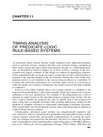
11.1.2 The Rete Network
Of these three phases, the match phase is by far the most expensive, accounting for
more than 90 percent of execution time in some experiments [Forgy, 1982; Gupta,
1987; Ishida, 1994]. Therefore, to maximize the efficiency of an OPS5 program, a
fast match algorithm is necessary. The Rete match algorithm was first introduced in
[Forgy, 1982] and it has become the standard sequential match algorithm. A new
version called Rete II was introduced in [Forgy, 1985].
The Rete algorithm compiles the LHS patterns of the production rules into a dis-
crimination network in the form of an augmented dataflow network [Miranker, 1987].
The state of all matches is stored in the memory nodes of the Rete network. Since a
limited number of changes are made to the working memory after the firing of a rule
instantiation, only a small part of the state of all matches needs to be changed. Thus,
(p p1
(c1 ^a1 <x> ^a2 10)
(c2 ^a1 <x>)
-->
(remove 2))
(p p2
(c1 ^a1 <y> ^a2 10)
(c3 ^a1 2 ^a2 <y>)
-(c4 ^a1 <y>)

-->
(modify 1 ^attri 4))
root
class=c2 class=c1 class=c3
class=c4

a2=10 a1=2
alpha
memory
node
and-node
terminal-node
p1
beta memory
node
alpha
memory
node
alpha
memory
node
alpha
memory
node
not-node
terminal-node
p2
and-node
Constant-test
nodes

Figure 11.1 An example of a Rete network.
CHENG–TSAI TIMING ANALYSIS METHODOLOGY
373
rather than checking every rule to determine which rules are matched by the WM in
each recognize–act cycle, Rete maintains a list of matched rules and determines how
these matches change due to the modification of the WM by the firing of a rule in-
stantiation. The top portion of the Rete network contains chains of tests that perform
the select operations. Tokens passing through these chains partially match a partic-
ular condition element and are stored in alpha-memory nodes. The alpha-memory
nodes are connected to the two input nodes that find the partial binding between con-
dition elements. Tokens with consistent variable bindings are stored in beta-memory
nodes. At the end of the two input nodes are the terminal nodes, which signify that
a consistent binding for a particular rule is found. The terminal nodes send the rule
bindings to the conflict set. An example of a Rete network is shown in Figure 11.1.
11.2 CHENG–TSAI TIMING ANALYSIS METHODOLOGY
11.2.1 Static Analysis of Control Paths in OPS5
Several graphical representations of procedural programs have been developed for
testing and debugging purposes. An intuitive representation is a physical rule flow
graph. In such a graph, nodes represent rules, and an edge from node a to b implies
rule b is executed immediately after rule a is executed. This graph is not appropriate
for rule-based programs because the execution order of OPS5 programs cannot be
determined statically. On the other hand, the control flow of rule-based programs
should be thought of in terms of logical paths. A physical rule flow graph does not
present the most appropriate abstraction. Another approach to represent the control
paths is a causality graph. Here, too, nodes represent rules, but an edge from node
a to node b implies rule a causes rule b to fire. The RHS assertions of rule a match
all the LHS condition elements of rule b. This graph is not sufficient to capture
all the logical paths since the LHS conditions of a rule are usually generated from
the RHS actions of many rules; that is, a combination of several rules may “cause”
another single rule to fire. This leads to the definition of a graph called the enable

rule (ER) graph, which is adapted from [Cheng and Wang, 1990] and [Kiper, 1992].
The control information among rules in an OPS5 program is represented by the ER
graph. To define the ER graph, we need to first define the state-space graph.
Definition 1. The state-space graph of an OPS5 program is a labeled directed graph
G = (V, E). V is a distinct set of nodes, each of which represents a distinct set of
WMEs. We say that a rule is enabled at node i if and only if its enabling condition is
satisfied by the WMEs at node i . E is a set of edges, each of which denotes the firing
of a rule such that an edge (i, j) connects node i to node j if and only if a rule R is
enabled at node i, and firing R will modify the WM to become the set of WMEs at
node j .
Definition 2. Rule a is said to potentially enable rule b if and only if there exists
at least one reachable state in the state-space graph of the program where (1) the
374
TIMING ANALYSIS OF PREDICATE-LOGIC RULE-BASED SYSTEMS
(c1 ^a1 2 ^a2 3)
(c2 ^b1 5)
(c1 ^a1 4 ^a2 3)
(c2 ^b1 3)
(c1 ^a1 3 ^a2 3)(c1 ^a1 5 ^a2 3)
(p r1
(c1 ^a1 <x> ^a2 3)
(c2 ^b1 { <y> <> <x> } )
-->
(modify 1 ^a1 <y>)
(remove 2))
(p r1
(c1 ^a1 <x> ^a2 3)
(c2 ^b1 { <y> <> <x> })
-->
(modify 1 ^a1 <y>)

(remove 2))
(p r3
(c1 ^a1 2 ^a2 <x>)
(c2 ^b1 5)
-(c1 ^a1 <x>)
-->
(modify 1 ^a1 4)
(modify 2 <x>))
(p r2
(c1 ^a1 5 ^a2 <x>)
-->
(modify 1 ^a1 <x>))
Figure 11.2 State-space graph of an OPS5 program.
enabling condition of rule b is false, (2) the enabling condition of rule a is true, and
(3) firing rule a causes the enabling condition of rule b to become true.
Figure 11.2 shows the state-space graph of an OPS5 program. Rule r 1 potentially
enables rule r 2, and rule r 3 potentially enables rule r 1. Suppose we have m different
attributes in all classes, each attribute has n data items, and each WME is a unit in the
WM, then we have n
m
possible WMEs. In the state-space graph, 2
n
m
states would
exist.
Since the state-space graph cannot be derived without running the program for all
allowable initial states, we use symbolic pattern matching to determine the poten-
tially enabling relation between rules. Rule a potentially enables rule b if and only
if the symbolic form of a WME modified by the actions in rule a matches one of
the enabling condition elements of rule b. Here the symbolic form represents a set of

WMEs and is of the form
(classname ^attribute1 v1 ^attribute2 v2 ... ^attributen vn)
where v1, v2 ..., and vn are either variables or constant values and each attribute
can be omitted. For example,
(class ^a1 3 ^a2 <x>)
can be a symbolic form of the
following WMEs.
(class ^a1 3 ^a2 4)
(class ^a1 3 ^a2 8 ^a3 4)
(class ^a1 3 ^a2 <y> ^a3 <z>)
CHENG–TSAI TIMING ANALYSIS METHODOLOGY
375
Note that to determine with certainty whether a rule enables rather than poten-
tially enables another rule, and thus determine whether the condition elements of a
rule actually have a matching, would require us to know the contents of the working
memory at run-time. This a priori knowledge of the WM cannot be obtained stati-
cally. Therefore, the above approximation of the potentially enabling relation is used
instead. Example 1 illustrates the potentially enabling relation. Rule a potentially
enables rule b because the first action of rule a creates a WME
(class c ^c1 off ^c2
<x>)
, which symbolically matches the enabling condition
(class c ^c1 <y>)
of rule b.
Notice, incidentally, that the second action of rule a does not match the first enabling
condition
(class a ^a1 <x> ^a2 off)
of rule b because variable
<y>
ranges in

<<open
close>>
.
Example 1. An example of a potentially enabling b.
(p a
(class_a ^a1 <x> ^a2 3)
(class_b ^b1 <x> ^b2 {<y> <<open close>>})
-->
(make class_c ^c1 off ^c2 <x>)
(modify 1 ^a2 <y>))
(p b
(class_a ^a1 <x> ^a2 off)
(class_c ^c1 <y>)
-->
(modify 1 ^a2 open))
The symbolic matching method actually detects the enabling relation by checking
the attribute ranges. This information can be found by analyzing the semantics of the
rules.
Definition 3. The (ER) graph of a set of rules is a labeled directed graph G =
(V , E). V is a set of vertices such that there is a vertex for each rule. E is a set of
edges such that an edge connects vertex a to vertex b if and only if rule a potentially
enables rule b.
Note that an edge from a to b in the ER graph does not mean that rule b will fire
immediately after rule a. The fact that rule b is potentially enabled only implies that
the instantiation of rule b may be added to the conflict set to be fired.
The previous analysis is useful since it does not require us to know the contents
of working memory that cannot be obtained statically.
11.2.2 Termination Analysis
As described in the introduction, the upper bound on a real-time expert system’s ex-
ecution time cannot exceed the length of the period between two consecutive sensor

input readings [Cheng et al., 1993; Chen and Cheng, 1995b]. Therefore, our goal is
to determine before run-time a tight upper bound on the execution time of the expert
system in every invocation following each reading of sensor input values. The first
analysis step is to determine whether the expert system terminates. Since a rule-based
expert system program is data-driven, it is not designed for all possible data domains.
Certain input data are required to direct the control flows in the program. Many con-
376
TIMING ANALYSIS OF PREDICATE-LOGIC RULE-BASED SYSTEMS
trol techniques are implemented in this manner, and the absence of certain WMEs or
a specific ordering of WMEs is required to generate the initial WM. If these WMEs
are not present in the expected data domain, abnormal program behavior will occur,
usually leading to a cycle in the program flow.
Ullman [Ullman and Van Gelder, 1988] studied recursive relations and described
termination conditions in backward-chaining programs. Here, we consider the ter-
mination conditions for forward-chaining rule-based programs. We examine the ER
graph of an OPS5 program to detect the termination conditions. If the OPS5 program
is found not to terminate for all initial program states, the culprit conditions that cause
nontermination are extracted to assist programmers in correcting the program.
Termination Detection
An OPS5 program is terminating if the maximal num-
ber of its rule firings is finite. Thus the maximal number of times a rule in a termi-
nating program can fire is also finite. A rule is said to be terminating if its number of
firings is always finite. To detect program termination, we use the ER graph, which
provides information about the logical paths of an OPS5 program. In particular, we
use this graph to trace the control flows of the program. Because we know the poten-
tially enabling relation between rules, we can detect if the firing of each rule in an
OPS5 program can terminate. The following definitions are needed to describe the
conditions under which a rule will terminate.
Definition 4. Suppose rule a potentially enables rule b. Then there is an edge from
node a to node b in the ER graph. A matched condition element of rule b is one of

the enabling condition elements of rule b, which may be matched by executing an
action of rule a. Here, rule a is called the enabling rule of the matched condition
element.
Definition 5. An unmatched condition element is one of the enabling condition ele-
ments of a rule, which cannot be matched by firing any rule.
Note that an unmatched condition can still be matched by the initial working
memory.
Example 2. Matched and unmatched condition elements
(p a
(c1 ^a1 5)
(c2 ^a2 <x> ^a3 2)
-->
(modify 2 ^a2 3))
(p b
(c2 ^a2 <x>)
(c3 ^a4 <x> ^a5 <y>)
-->
(modify 1 ^a2 <y>))
CHENG–TSAI TIMING ANALYSIS METHODOLOGY
377
In example 2, suppose the firing of any other rule cannot match the second condi-
tion element of rule a. In the ER graph, rule b will potentially enable rule a.Thefirst
condition element
(c2 ^a2 <x>)
of rule a is a matched condition element because it
may be matched by firing rule b. The second condition element
(c3 ^a4 <x> ^a5 <y>)
of rule a is an unmatched condition element because it cannot be matched by firing
other rules.
An important property of OPS5 rule-based systems is called refraction, which

ensures that the same instantiation is never executed more than once. Two instantia-
tions are considered the same if they have the same rule name and the same WMEs
matching to the same condition elements.
Next, we derive a theorem to detect the termination of a program. One way to pre-
dict the termination condition is to make sure that every state in the state-space graph
cannot be reached more than once. However, since it is computationally expensive
to expand the whole state-space graph, we use the ER graph to detect this property.
Theorem 1. A rule r will terminate (terminate in finite firings) if one of the follow-
ing conditions holds:
C0. No rule potentially enables rule r.
C1. The actions of rule r modify or remove at least one of the unmatched condi-
tion elements of rule r.
C2. The actions of rule r modify or remove at least one of the matched condition
elements of rule r , and all of the enabling rules of the matched condition
elements can terminate in finite firings.
C3. Every rule that enables rule r can terminate in finite firings.
Note that condition (C1) is not necessary for OPS5 rules because refraction in
OPS5 prevents a rule from firing again immediately after firing once. Also, if rule r
is self-enabling, condition (C2) is not satisfied.
Proof
C0. If no rule potentially enables rule r, the instantiations of rule r can be formed
only from the initial WM. Since the number of WMEs in the initial WM is
finite, the number of firings of rule r is also finite.
C1. Since the firing of any rule cannot match the unmatched condition elements,
the only WMEs that can match the unmatched condition elements are the
initial WMEs. Moreover, since the actions of rule r change the contents of
these WMEs, the WMEs cannot match the unmatched condition elements
again after rule r is fired. Otherwise, the unmatched condition elements will
be matched by firing rule r . This contradicts the definition of unmatched
condition elements. Each initial WME matching the unmatched condition

element can cause rule r to fire at most once since we have a finite number
of initial WMEs. Thus rule r can terminate in finite firings.
378
TIMING ANALYSIS OF PREDICATE-LOGIC RULE-BASED SYSTEMS
C2. Since the enabling rules of the matched condition elements can terminate in
finite firings, by removing these rules the matched condition elements can
be treated as unmatched condition elements. According to (C1), rule r can
terminate in finite firings.
C3. All rules that enable rule r can terminate in finite firings. After these rules
terminate, no other rule can trigger rule r to fire. Thus rule r can terminate
as well.
Example 3. A rule can terminate in finite firings.
(p a
(c1 ^a1 1 ^a2 <x>)
(c2 ^a1 4 ^a2 <x>)
-->
(modify 2 ^a1 3))
In example 3, suppose the second condition element
(c2 ^a1 4 ^a2 <x>)
cannot
be matched by firing any rule, including this rule itself. Then this condition element
is an unmatched condition element. Suppose three WMEs are in the initial work-
ing memory matching this condition element. Then this condition element can be
matched by at most three WMEs. The actions of rule a modify these three WMEs
when rule a fires. As a result, rule a can fire at most three times.
Example 4. Two rules with a cycle embedded.
(p p1
(class1 ^a11 { <x> <>1})
(class2 ^a21 <y>)
-->

(modify 1 ^a11 <y>))
(p p2
(class1 ^a11 <x>)
(class2 ^a21 { <x> <<23>>}^a22 <y>)
-->
(modify 1 ^a11 <y>))
Example 5. Example 4 with modified variables.
(p p1
(class1 ^a11 { <x-1> <> 1 } )
(class2 ^a21 <y-1>)
-->
(modify 1 ^a11 <y-1>))
(p p2
(class1 ^a11 <x-2>)
(class2 ^a21 { <x-2> << 2 3 >> } ^a22 <y-2>)
-->
(modify 1 ^a11 <y-2>))
CHENG–TSAI TIMING ANALYSIS METHODOLOGY
379
Enabling Conditions of a Cycle
We use the above termination-detection al-
gorithm to determine whether an OPS5 program always terminates in bounded time
by inspecting the ER graph of the program. If no cycle exists in the ER graph or
every cycle can be broken, that is, each cycle can be exited as a result of the firing
of a rule that disables one or more LHSs of rules in this cycle [Cheng et al., 1993],
then the firings of every rule in the OPS5 program are finite, and thus termination
is detected. However, if the OPS5 program is not detected to terminate for all initial
program states, then the culprit conditions that cause nontermination are extracted to
assist programmers in correcting the program. This is done by inspecting the cycles
with no exit conditions in the ER graph. Again, note that cycles composed entirely

of rules that terminate in finite firings (and hence have exit conditions) do not need
to be examined.
We now discuss the conditions under which a cyclic sequence of rule firings oc-
curs. Suppose rules p
1
, p
2
..., p
n
form a cycle in the ER graph, W is a set of WMEs,
and W causes rules p
1
, p
2
..., p
n
to fire in that order. If firing p
1
, p
2
..., p
n
in that
order will produce W again, then W is called an enabling condition of the cycle. We
can use symbolic tracing to find W if the data of each attribute are literal. Example 4
illustrates the idea.
Rules p
1
and p
2

form a cycle in the ER graph. To distinguish different variables in
different rules, we assign different names to variables. Thus, the program is rewritten
as in example 5. A symbol table is built for each variable, which is bound accord-
ing to the semantics of the enabling conditions. Here, Table A is the symbol table,
where the Binding Space refers to the restrictions imposed by the semantics of the
constraints on the variables from the rule conditions.
In order to derive an acceptable enabling condition of the cycle, the algorithm be-
low first postulates it to be the set of all enabling conditions of the rules of the cycle.
Then it removes redundant conditions to arrive at a condition suitable for examina-
tion by the programmer, to see if the cycle should be broken by introducing further
conditions into the LHSs of the rule. Thus W is
(class1 ^a11 <x-1>)
(class2 ^a21 <y-1>)
(class1 ^a11 <x-2>)
(class2 ^a21 <x-2> ^a22 <y-2>)
Each variable occurs once in the symbol table.
Now we trace the execution by firing p
1
first; p
1
enables p
2
by matching the first
condition. Since the first condition of rule p
2
can be generated from rule p
1
, it can
TABLE A
Variable Binding space

x-1 <>1
y-1 none
x-2 2,3
y-2 none
TABLE B
Variable Binding space
x-1 <>1
y-1 2,3
x-2 2,3
y-2 none
TABLE C
Variable Binding space
x-1 <>1
y-1 2,3
x-2 2,3
y-2 <>1
380
TIMING ANALYSIS OF PREDICATE-LOGIC RULE-BASED SYSTEMS
be removed from W . Variable x-2 is now replaced by y-1. W is
(class1 ^a11 <x-1>)
(class2 ^a21 <y-1>)
(class2 ^a21 <y-1> ^a22 <y-2>)
Since x-2 is bound with 2 and 3, y-1 is bound with the same items. The symbol
table is modified (Table B). In general, the conjunction of the binding-space restric-
tions is substituted.
After executing the action of rule p
2
, W is now
(class1 ^a11 <y-2>)
(class2 ^a21 <y-1>)

(class2 ^a21 <y-1> ^a22 <y-2>)
To make this WM trigger p
1
and p
2
in that order again, the WME
(class1 ^a11
<y-2>)
must match the first condition of p
1
. Thus variable y-2 is bound with the
binding space of x-1. Table C is the symbol table. W is
(class1 ^a11 <y-2>)
(class2 ^a21 <y-1>)
(class2 ^a21 <y-1> ^a22 <y-2>)
where y-2<>1 and y-1=2,3
The detailed algorithm for detecting the enabling conditions of cycles is described
next.
Algorithm 1. The detection of enabling conditions of cycles.
Premise: The data domain of each attribute is literal.
Purpose: Rules p
1
, p
2
..., p
n
form a cycle in the ER graph. Find a set of WMEs,
W , that fires p
1
, p

2
..., p
n
in that order such that these firings cannot termi-
nate in finite firings.
1. Assign different names to the variables in different rules.
2. Initialize W to the set of all enabling conditions of p
1
, p
2
..., p
n
.
3. Build a symbol table for variables. Each variable’s binding set is limited to the
restriction specified in the rule enabling conditions.
4. Simulate the firing of p
1
, p
2
..., p
n
in that order.
Each enabling condition of rule p
i
is matched from the initial WM, unless
it can be generated from rule p
i−1
.
If the enabling condition element w of rule p
i

can be generated by firing
p
i−1
, then remove w from W . Substitute p
i−1
’s variables v
i−1
for correspond-
ing variables v
i
in p
i
.
Modify v
i−1
’s binding space in the symbol table to the conjunction of the
restrictions on v
i
and v
i−1
.
CHENG–TSAI TIMING ANALYSIS METHODOLOGY
381
5. If p
1
’s enabling condition elements can be generated by p
n
, substitute p
n
’s

variables v
n
for corresponding variables v
1
in p
1
. Modify v
n
’s binding space
in the symbol table.
6. In steps 4 and 5, while substituting p
i−1
’s variables for p
i
’s variables, check
the intersection of the binding spaces of p
i
’s and p
i−1
’s variables. If the in-
tersection is empty, then terminate the algorithm: the loops terminates in finite
firings.
7. Suppose W
n
is the WM after firing p
1
, p
2
..., p
n

.IfW
n
can match W , then
W is an enabling condition of the cycle p
1
, p
2
..., p
n
.
Note that certain conditions are subsets of others, as explained in section 4.4.
Prevention of Cycles
If the OPS5 program is not detected to terminate for all
initial program states, then the culprit conditions that cause nontermination are used
to assist programmers in correcting the program. After detecting the enabling condi-
tions, W , of a cycle, we add rule r

, with W as the enabling conditions of r

. By doing
so, once the working memory has the WMEs matching the enabling conditions of a
cycle, the control flow can be switched from the cycle to r

. In example 4, r

is
(p loop-rule1
(class1 ^a11 { <y-2> <>1 } )
(class2 ^a21 { <y-1> << 2 3 >> } )
(class2 ^a21 <y-1> ^a22 <y-2>)

-->
action ...
If the cycle is not an infinite loop or desirable (e.g., in periodic control and mon-
itoring applications), we may not want to add rule r

. The action of r

, determined
by the application, depends on how the application needs to react when the program
flow is going to enter a cycle. The simplest way to escape from the cycles is to halt.
To ensure the program flow switches out of the cycles, the extra rules r

should
have higher priorities than the regular ones. To achieve this goal, we use the MEA
control strategy and modify the enabling conditions of each regular rule.
At the beginning of the program, two WMEs are added to the WM and the MEA
strategy is enforced.
(startup
......
(strategy mea)
(make control ^rule regular)
(make control ^rule extra))
The condition
(control ^rule regular)
is added to each regular rule as the first
enabling condition element.
(control ^rule extra)
is added to each extra rule as the
first enabling condition element too. Since the MEA strategy is enforced, the order
of instantiations is based on the recency of the first time tag. The recency of the

condition
(control ^rule regular)
is lower than that of the condition
(control ^rule
382
TIMING ANALYSIS OF PREDICATE-LOGIC RULE-BASED SYSTEMS
extra)
. Thus, the instantiations of the extra rules are chosen for execution earlier than
those of the regular rules. Example 6 is the modified result of example 4.
Example 6. The modified result of example 4.
(startup
(strategy mea)
(make control ^rule regular)
(make control ^rule extra))
(p p1
(control ^rule regular)
(class1 ^a11 { <x> <>1})
(class2 ^a21 <y>)
-->
(modify 2 ^a11 <y>))
(p p2
(control ^rule regular)
(class1 ^a11 <x>)
(class2 ^a21 { <x> <<23>>}^a22 <y>)
-->
(modify 2 ^a11 <y>))
(p loop-rule1
(control ^rule extra)
(class1 ^a11 { <y-2> <> 1 } )
(class2 ^a21 { <y-1> << 2 3 >> } )

(class2 ^a21 <y-1> ^a22 <y-2>)
-->
(halt))
Usually, a cycle is not expected for an application. Thus, once the entrance of a
cycle is detected, the program can be abandoned. Hence, after all cycles in the ER
graph are found, the program is guaranteed to terminate. In example 6, the action of
the extra rule can be
(remove 2 3 4)
Since the WMEs that match the enabling condition of a cycle are removed, the
instantiations in the cycle are also removed. Then, other instantiations in the agenda
can be triggered to fire.
Another example of program modification is shown in the analysis of the Space
Shuttle Orbital Maneuvering and Reaction Control Systems’ Valve and Switch Clas-
sification Expert System (OMS) [Barry and Lowe, 1990]. A non-terminating rule is
modified in order to break a cycle, thus guaranteeing the termination of this rule and
the program.
Program Refinement
Due to its complexity, the ER graph usually contains
many cycles. Furthermore, even for a single cycle, more than one enabling condition
may exist to trigger the cycle. This leads to a large number of extra rules in the mod-
ified programs and thus reduces their run-time performance. To tackle this problem,
redundant conditions and rules must be removed after the modification.
CHENG–TSAI TIMING ANALYSIS METHODOLOGY
383
Redundant Conditions
In algorithm 1, after symbolic tracing, some variables
will be substituted and the binding spaces may be changed too. This may cause subset
relationships among the enabling condition elements of a cycle. In an extra rule, if
condition element C
i

is a subset of condition element C
j
, then C
j
can be omitted
to simplify the enabling condition. In example 6, the condition
(class2 ^a21 <y-1>
^a22 <y-2>)
is a subset of
(class2 ^a21 <y-1>)
. Hence,
(class2 ^a21 <y-1>)
can be
omitted.
(p loop-rule1
(control ^rule extra)
(class1 ^a11 { <y-2> <>1 } )
; (class2 ^a21 { <y-1> <<23>>}) ;omitted
(class2 ^a21 <y-1> << 2 3 >> ^a22 <y-2>)
-->
(halt))
Redundant Extra Rules
In certain situations, we can remove some extra rules
if the actions of these extra rules can be ignored. For example, extra rules with action
“halt” or “print” can be ignored. Since each cycle is analyzed independently, the
extra rules correspond to cycles with different enabling conditions. If the enabling
condition of rule r
i
is a subset of the enabling condition of rule r
j

, then rule r
i
can
be removed since firing r
i
will definitely fire r
j
. The cycling information of rule r
j
contains that of rule r
i
. Thus, it is sufficient to just provide more general information.
In many cases, if the set of nodes P
i
which forms a cycle C
i
is a subset of the set
P
j
which forms a cycle C
j
, then the enabling condition of C
j
is a subset of C
i
’s
enabling condition. The situation becomes apparent when the cycle consists of many
nodes. Hence, we can expect to remove the extra rules whose enabling conditions
are derived from large cycles.
In example 7, the first and third condition elements of rule 1 are identical to the

first and fourth condition elements, respectively, of rule 3. WMEs matching the sec-
ond condition element of rule 3 also match the second condition element of rule 1,
but not vice versa. The third condition element of rule 3 is not in rule 1, making the
LHS of rule 3 more restrictive than the LHS of rule 1. Thus the enabling condition of
rule 3 is a subset of the enabling condition of rule 1. Similarly, the first, second, and
fourth condition elements of rule 2 are identical to the first, second, and fifth condi-
tion elements, respectively, of rule 4. WMEs matching the third condition element
of rule 4 also match the third condition element of rule 2, but not vice versa. The
fourth condition element of rule 4 is not in rule 2, making the LHS of rule 4 more
restrictive than the LHS of rule 2. Thus the enabling condition of rule 4 is a subset
of the enabling condition of rule 2. Therefore, rules 3 and 4 can be removed.
Example 7. Redundant rules.
(p 1
(control ^rule extra)
(class1 ^a13 { <y-1> <> 1 } )
(class2 ^a22 <y-1>)
384
TIMING ANALYSIS OF PREDICATE-LOGIC RULE-BASED SYSTEMS
-->
action ...
(p 2
(control ^rule extra)
(class1 ^a13 { <x-1> <> 1 } )
(class2 ^a22 <y-1>)
(class4 ^a41 2 ^a42 <x-3>)
-->
action ...
(p 3 ; redundant rule of rule 1
(control ^rule extra)
(class1 ^a13 { <y-1> << 2 3 >> } )

(class4 ^a41 { <y-4> <> 1 } ^a42 <y-1>)
(class2 ^a22 <y-1>)
-->
action ...
(p 4 ; redundant rule of rule 2
(control ^rule extra)
(class1 ^a13 { <x-1> <> 1} )
(class2 ^a22 { <y-1> << 2 3 >> }
(class4 ^a41 <y-4> ^a42 <y-1>)
(class4 ^a41 2 ^a42 <x-3>)
-->
action ...
An Example
Now we apply our technique to a complete example.
Example 8. An OPS5 program with cycles embedded in the ER graph.
(p p1
(class1 ^a13 { <x> <> 1 } )
(class2 ^a22 <y>)
-->
(modify 1 ^a13 <y>))
(p p2
(class3 ^a31 <x> ^a32 <y>)
(class4 ^a41 <x> ^a42 <y>)
-->
(modify 1 ^a31 2 ^a32 <x>)
(make class1 ^a11 1 ^a12 2 ^a13 3))
(p p3
(class1 ^a11 <x> ^a12 <y>)
(class4 ^a41 2 ^a42 <x>)
-->

(modify 1 ^a11 <y>))
(p p4
(class1 ^a13 { <x> << 2 3 >> } )
(class4 ^a41 <y> ^a42 <x>)
-->
(modify 1 ^a13 <y>))
CHENG–TSAI TIMING ANALYSIS METHODOLOGY
385
(p p5
(class1 ^a11 <x>)
(class3 ^a31 1 ^a32 <y>)
-->
(modify 2 ^a31 2 ^a32 <x>)
(make class2 ^a21 2 ^a22 3))
First, we detect if the program can terminate in finite firings. We find rule p5 can
terminate since it contains an unmatched condition. Next, the enabling condition of
each cycle is found and extra rules are added to the program (Example 9). Here, the
actions of all extra rules are
halt
. Hence, we remove the redundant rules without
considering the interference among the extra rules. After removing the redundant
rules, the number of extra rules is reduced from 16 to 9.
Example 9. Extra rules of example 8 (including redundant rules).
(p loop-rule1 ;cycle: 4
(control ^rule extra)
(class1 ^a13 {<y-4> <<32>>})
(class4 ^a41 <y-4> ^a42 <y-4> )
-->
; cycle information
(p loop-rule2 ;cycle: 3

(control ^rule extra)
(class1 ^a11 <y-3> ^a12 <y-3> )
(class4 ^a41 2 ^a42 <y-3> )
-->
; cycle information
(p loop-rule3 ;cycle: 2
(control ^rule extra)
(class3 ^a31 2 ^a32 2)
(class4 ^a41 2 ^a42 2)
-->
; cycle information
(p loop-rule4 ;cycle: 1
(control ^rule extra)
(class1 ^a13 {<y-1> <> 1} )
(class2 ^a22 <y-1> )
-->
; cycle information
(p loop-rule5 ;cycle: 3 4
(control ^rule extra)
(class1 ^a11 <x-3> ^a12 <y-3> )
(class4 ^a41 2 ^a42 <x-3> )
(class4 ^a41 <y-4> ^a42 {<x-4> << 3 2 >>} )
-->
; cycle information
(p loop-rule6 ;cycle: 1 4
(control ^rule extra)
(class1 ^a13 {<y-4> <> 1} )
(class2 ^a22 {<y-1> <<32>>})
(class4 ^a41 <y-4> ^a42 <y-1> )
-->

; cycle information
(p loop-rule7 ;cycle: 4 3
(control ^rule extra)
(class1 ^a13 <x-4> << 3 2 >> )
(class4 ^a41 <y-4> ^a42 <x-4> )
(class4 ^a41 2 ^a42 <x-3> )
-->
; cycle information
386
TIMING ANALYSIS OF PREDICATE-LOGIC RULE-BASED SYSTEMS
(p loop-rule8 ;cycle: 1 3
(control ^rule extra)
(class1 ^a13 {<x-1> <> 1} )
(class2 ^a22 <y-1> )
(class4 ^a41 2 ^a42 <x-3> )
-->
; cycle information
(p loop-rule9 ;cycle: 4 1
(control ^rule extra) ;redundant with loop-rule1
(class1 ^a13 {<y-1> << 3 2>>} )
(class4 ^a41 {<y-4> <> 1} ^a42 <y-1> )
(class2 ^a22 <y-1> )
-->
; cycle information
(p loop-rule10 ;cycle: 3 1
(control ^rule extra)
(class1 ^a11 <x-3> ^a12 <y-3> )
(class4 ^a41 2 ^a42 <x-3> )
(class2 ^a22 <y-1> )
-->

; cycle information
(p loop-rule11 ;cycle: 1 4 3
(control ^rule extra) ;redundant with loop-rule8
(class1 ^a13 {<x-1> <>1} )
(class2 ^a22 {<y-1> <<32>>})
(class4 ^a41 <y-4> ^a42 <y-1> )
(class4 ^a41 2 ^a42 <x-3> )
-->
; cycle information
(p loop-rule12 ;cycle: 3 4 1
(control ^rule extra) ;redundant with loop-rule10
(class1 ^a11 <x-3> ^a12 <y-3> )
(class4 ^a41 2 ^a42 <x-3> )
(class4 ^a41 {<y-4> <> 1} ^a42 {<x-4> <<32>>})
(class2 ^a22 <y-1> )
-->
; cycle information
(p loop-rule13 ;cycle: 1 3 4
(control ^rule extra) ;redundant with loop-rule8
(class1 ^a13 {<y-4> <> 1} )
(class2 ^a22 <y-1> )
(class4 ^a41 2 ^a42 <x-3> )
(class4 ^a41 <y-4> ^a42 {<x-4> << 3 2 >>} )
-->
; cycle information
(p loop-rule14 ;cycle: 4 3 1
(control ^rule extra) ;redundant with loop-rule7
(class1 ^a13 {<y-1> <<32>>})
(class4 ^a41 <y-4> ^a42 <y-1> )
(class4 ^a41 2 ^a42 <x-3> )

(class2 ^a22 <y-1> )
-->
; cycle information
(p loop-rule15 ;cycle: 3 1 4
(control ^rule extra) ;redundant with loop-rule5
(class1 ^a11 <x-3> ^a12 <y-3> )
(class4 ^a41 2 ^a42 <x-3> )
(class2 ^a22 {<y-1> <<32>>})
(class4 ^a41 <y-4> ^a42 <y-1> )
-->
; cycle information
(p loop-rule16 ;cycle: 4 1 3
(control ^rule extra) ;redundant with loop-rule7
(class1 ^a13 {<x-4> <<32>>})
(class4 ^a41 {<y-4> <> 1} ^a42 <x-4> )
(class2 ^a22 <y-1> )
(class4 ^a41 2 ^a42 <x-3> )
-->
; cycle information
CHENG–TSAI TIMING ANALYSIS METHODOLOGY
387
Implementation and Complexity
For an OPS5 program with n rules, poten-
tially O(n!) cycles are embedded in the ER graph. However, we found that cycles do
not contain a large number of nodes in actual real-time expert systems we examined.
If it is detected that no path contains m nodes in the ER graph, there is no need to
test cycles with more than m nodes. This reduces both the computational complexity
and the memory space.
To further reduce the computation time in identifying cycles, we store information
about rules that do not form a path in certain orders. This non-path is called an

impossible path. If there is no path consisting of rules p
1
, p
2
..., p
n
executing in this
order, then there is no cycle containing these rules. Thus, we do not need to examine
the cycles with an embedded path consisting of the rules in the above order (an
impossible path). Since the ER graph actually represents all possible paths between
two rules, we can construct a linear list to store all impossible paths with more than
two rules. Since storage of these impossible paths requires space, we are in fact
trading space with time. In our tool, we store impossible paths with up to nine nodes.
This tool has been implemented on a DEC 5000/240 workstation running
RISC/Ultrix. Two real-world expert systems are examined. Ongoing work applies
this tool to more actual and synthetic OPS5 expert systems in order to evaluate the
run-time performance and scalability of this tool.
Industrial Example: Experiment on the ISA Expert System
The purpose
of the Integrated Status Assessment (ISA) Expert System [Marsh, 1988] is to deter-
mine the faulty components in a network. It contains 15 production rules and some
Lisp function definitions. A component can be either an entity (node) or a relation-
ship (link). A relationship is a directed edge connecting two entities. Components
are in one of three states: nominal, suspect, or failed. A failed entity can be replaced
by an available backup entity. This expert system makes use of simple strategies to
trace failed components in a network.
One rule is found to terminate in a finite number of firings. One hundred twenty
five cycles are detected. After removing the redundant rules, four cycles remain.
Industrial Example: Experiment on the OMS Expert System
The purpose

of the OMS Expert System [Barry and Lowe, 1990] is to classify setting valves and
switches. It recognizes special patterns of settings and creates intermediate asser-
tions. With settings and new assertions, it infers more and creates more assertions
until no more assertions can be derived. Finally, the settings and assertions are com-
pared with the expected values supplied by the user. All matches or mismatches are
reported.
No rule is reported to terminate in finite firings. However, after checking all possi-
ble paths, only one cycle is found. The enabling condition of the cycle, shown below,
is in rule
loop-rule1
.
(control ^rule extra)
(device ^mode {<x-4> <> void } ^domain <y-4>
^compnt <v-4> ^desc {<w-4> << closed open >>} )
(valve_groups ^vtype <v-4> ^valve_a <v-4> ^valve_b <v-4> )
388
TIMING ANALYSIS OF PREDICATE-LOGIC RULE-BASED SYSTEMS
This cycle contains only the fourth rule. It implies the other rules can terminate in
finite firings. The fourth rule is
(p check-group
(device ^mode { <x> <> void } ^domain <y>
^compnt <z1> ^desc { <w> << open closed >> })
(device ^mode <x> ^domain <y> ^compnt <z2> ^desc <w>)
(valve_groups ^vtype <v> ^valve_a <z1> ^valve_b <z2>)
-->
(modify 1 ^compnt <v>)
(modify 2 ^mode void))
We then examine the non-terminating rule with the enabling condition of the
cycle. We find that the program flow can enter the cycle when variable
<z1>

is equal
to variable
<z2>
in the rule
check-group
. This situation is not expected as a normal
execution flow. Hence, we modify the LHS of this rule such that variable
<z1>
is not
equal to variable
<z2>
.
(p check-group
(device ^mode { <x> <> void } ^domain <y>
^compnt <z1> ^desc { <w> << open closed >> })
(device ^mode <x> ^domain <y> ^compnt { <z2> <> <z1> } ^desc <w>)
(valve_groups ^vtype <v> ^valve_a <z1> ^valve_b <z2>)
-->
(modify 1 ^compnt <v>)
(modify 2 ^mode void))
This modification breaks the cycle, thus guaranteeing the termination of this rule
and the program. In the next section, we introduce techniques for determining the
execution time of OPS5 programs.
11.2.3 Timing Analysis
Now we introduce techniques for analyzing the timing properties of OPS5 programs
and discuss a static-analytic method to predict the timing bound on program execu-
tion time. The ER graph is the basic structure of our static analysis. We predict the
timing in terms of the number of rule firings. Similar work has been done for MRL
in [Wang and Mok, 1993]. We will indicate the problems of static analysis and de-
scribe a tool to facilitate the timing analysis and to assist programmers in analyzing

run-time performance.
Before we analyze the problem, we need to make the following assumptions:
•
The program can terminate.
•
The data domains of all attributes are finite.
•
No duplicate WMEs are in the WM.
The first assumption is obvious since no timing bound can be found for a program
with infinite firings. The second assumption is based on the fact that the analysis
CHENG–TSAI TIMING ANALYSIS METHODOLOGY
389
problem is in general undecidable for programs with infinite domains. The third as-
sumption is actually an extension of the second assumption. Unlike MRL, OPS5’s
WMEs are identified not only by their contents but also by their time tags. Thus,
the following two WMEs are identified as different items in OPS5; the first WME is
generated earlier than the second WME. However, identical WMEs cannot co-exist
in the WM in MRL.
time tag WMEs
___________________________________
#3 (class ^a1 3 ^a2 4)
#6 (class ^a1 3 ^a2 4)
An OPS5 system can use a hash table to quickly locate the duplicate WMEs in the
WM and prevent redundancy in every cycle. If a set of WMEs satisfies the enabling
condition of the first firing rule, we can generate the same WMEs as many times as
we want. In other words, we can fire the first-firing rule as many times as we want.
This indicates that no upper bound exists for this rule’s firings, and thus the program
cannot terminate in a finite number of rule firings. Therefore, we need to enforce the
third assumption to facilitate our analysis.
11.2.4 Static Analysis

Prediction of the Number of Rule Firings
Since the execution of rule-based
programs is data-driven, the WM is used to predict the number of rule firings. To
predict the number of each rule’s firings, we estimate the number of instantiations in
the conflict set. The maximum number of instantiations of a rule can be estimated,
as in example 10.
Example 10. An example with a maximum number of instantiations.
(p a
(class_a ^a1 <x> ^a2 <y>)
(class_b ^b1 <x> ^b2 <z>)
(class_c ^c1 <z>)
-->
action without changing the instantiations of rule a ...
Assume the domains of
<x>
,
<y>
,and
<z>
contain at most x, y,andz instances,
respectively. Then, we have at most xyz instantiations of rule a in the conflict set.
Suppose the action of rule a does not remove any instantiations of rule a.There
are two situations in which rule a can be fired: (1) the initial WM contains rule a’s
instantiations, or (2) rule a is triggered by other rules.
In the first situation, we have at most xyz instantiations in the initial WM. Thus
rule a can fire at most xyz times before rule a is triggered by other rules.
In the second situation, another rule creates or modifies WME w which matches
one or more enabling condition elements of rule a. If the WME w matches the first
condition element,
(class a ^a1 <x> ^a2 <y>)

,atmostz of rule a instantiations will
390
TIMING ANALYSIS OF PREDICATE-LOGIC RULE-BASED SYSTEMS
be added into the conflict set because variables
<x>
and
<y>
are bound with the values
of w’s attributes. Thus rule a can fire at most z times before it is again triggered by
other rules. Similarly, if w matches
(class b ^b1 <x> ^b2 <z>)
or
(class c ^c1 <z>)
,
rule a can fire at most y or xy times, respectively, before another rule triggers rule a
again.
Also, the action part of a rule can affect the rule’s instantiations. For example, the
rule in example 10 can be
(p a
(class_a ^a1 <x> ^a2 <y>)
(class_b ^b1 <x> ^b2 <z>)
(class_c ^c1 <z>)
-->
(modify 3 ^c1 <y>))
Once the value of attribute
^c1
is changed, the instantiations associated with the
third condition element,
(class c ^c1 <z>)
, will be removed. Thus the maximum

number of firings is the number of instances of
<z>
, that is, z. Also, we reduce the
maximum number of firings from xyz to z. If rule a is triggered with the match of
the third condition element,
(class c ^c1 <z>)
, rule a can fire at most once before
another trigger.
Algorithm 2. Detection of the upper bound on the number of firings of rule r.
Premise: rule r can be detected to terminate in bounded time by using the termina-
tion detection algorithm 1.
Suppose we have up to I
r
instantiations of rule r in the initial WM. The upper
bound on the firings of rule r can be estimated according to the following conditions.
1. Rule r satisfies condition 1 of theorem 1: the upper bound on the firings of rule
r is I
r
. The maximum number of the initial WMEs is bounded by the domain
size of each attribute.
2. Rule r satisfies condition 2 of theorem 1: rules r
1
, r
2
,...,r
n
are enabling rules
of the matched condition elements of rule r . These rules can terminate in
f
1

, f
2
,..., f
n
firings, respectively. Rule r has at most I
1
, I
2
,...,I
n
instan-
tiations when triggered by r
1
, r
2
,...,r
n
. The upper bound on the number of
firings of rule r is
I
r
+
n

j=1
( f
j
× I
j
)

3. Rule r satisfies condition 3 of theorem 1: rules r
1
, r
2
,...,r
m
, which point
to rule r in the ER graph can terminate in f
1
, f
2
,..., f
m
firings, respec-
tively. Rule r has at most I
1
, I
2
,...,I
m
instantiations when triggered by
CHENG–TSAI TIMING ANALYSIS METHODOLOGY
391
r
1
, r
2
,...,r
m
. The upper bound on the number of firings of rule r is

I
r
+
m

j=1
( f
j
× I
j
)
Example 3 illustrates condition 1 of this algorithm. Example 11 illustrates condi-
tion 2 of this algorithm.
Example 11. A rule satisfying condition 2 of algorithm 2.
(p a
(c1 ^a1 1 ^a2 <y>)
(c2 ^a1 <x> ^a2 <y>)
-->
(modify 2 ^a2 <x>))
Suppose variables
<x>
and
<y>
have x and y items. The second condition element,
(c2 ^a1 <x> ^a2 <y>)
, is the matched condition element. The enabling rules of this
condition element can terminate in f
1
, f
2

,..., f
m
firings, respectively. We have up
to I
a
instantiations of rule a in the initial WM. Since the action does not affect the
WMEs that satisfy the first condition element,
(c1 ^a1 1 ^a2 <y>)
, there would be at
most y instantiations when this rule is triggered by one of the enabling rules. The
upper bound on the number of firings of rule a is
I
a
+
n

j=1
( f
j
× y)
Problems
Algorithm 2 is based on the ER graph. However, in the ER graph, we
use the symbolic matching method to detect the enabling relations. Since the contents
and interrelationship of WMEs cannot be determined statically, it is likely to cause a
pessimistic prediction, as in example 12.
Example 12. A rule with pessimistic estimation.
(p a
(class_a ^a1 7 ^a2 <x>)
(class_b ^b1 <x> ^b2 6)
-->

(make class_b ^b1 5 ^b2 4))
(p b
(class_a ^a1 { <x> <> <y> } ^a2 <y>)
-(class_a ^a1 <y> ^a2 <x>)
(class_b ^b1 <x> ^b2 <y>)
(class_b ^b1 <y> ^b2 <x>)
-->
(modify 3 ^b2 <x>))