Modeling, Measurement and Control P24

24

Intelligent
Soft-Computing

Techniques in Robotics

24.1 Introduction
24.2 Connectionist Approach in Robotics

Basic Concepts • Connectionist Models with
Applications in Robotics • Learning Principles
and Rules

24.3 Neural Network Issues in Robotics

Kinematic Robot Learning by Neural
Networks • Dynamic Robot Learning at the Executive
Control Level • Sensor-Based Robot Learning

24.4 Fuzzy Logic Approach

Introduction • Mathematical Foundations • Fuzzy
Controller • Direct Applications • Hybridization with
Model-Based Control

24.5 Neuro-Fuzzy Approach in Robotics
24.6 Genetic Approach in Robotics

24.7 Conclusion

24.1 Introduction

Robots and machines that perform various tasks in an intelligent and autonomous manner are
required in many contemporary technical systems. Autonomous robots have to perform various
anthropomorphic tasks in both unfamiliar or familiar working environments by themselves much
like humans. They have to be able to determine all possible actions in unpredictable dynamic
environments using information from various sensors. In advance, human operators can transfer to
robots the knowledge, experience, and skill to solve complex tasks. In the case of a robot performing
tasks in an unknown enviroment, the knowledge may not be sufficient. Hence, robots have to adapt
and be capable of acquiring new knowledge through learning. The basic components of robot
intelligence are actuation, perception, and control. Significant effort has been attempted to make
robots more intelligent by integrating advanced sensor systems as vision, tactile sensing, etc. But,
one of the ultimate and primary goals of contemporary robotics is development of intelligent
algorithms that can further improve the performance of robotic systems, using the above-mentioned
human intelligent functions.
Intelligent control is a new discipline that has emerged from the classical control disciplines
with primary research interest in specific kinds of technological systems (systems with recognition

Dustic M. Kati´c

Mihajlo Pupin Institute

Branko Karan

Mihajlo Pupin Institute

8596Ch24Frame Page 639 Tuesday, November 6, 2001 9:43 PM
© 2002 by CRC Press LLC

in the loop, systems with elements of learning and self-organization, systems that sometimes do
not allow for representation in a conventional form of differential and integral calculus). Intelligent
control studies high-level control in which control strategies are generated using human intelligent
functions such as perception, simultaneous utilization of a memory, association, reasoning, learning,
or multi-level decision making in response to fuzzy or qualitative commands. Also, one of the main
objectives of intelligent control is to design a system with acceptable performance characteristics
over a very wide range of structured and unstructured uncertainties.
The conditions for development of intelligent control techniques in robotics are different. It is
well known that classic model-based control algorithms for manipulation robots cannot provide
desirable solutions, because traditional control laws are, in most cases, based on a model with
incomplete information and partially known or inaccurately defined parameters. Classic algorithms
are extremely sensitive to the lack of sensor information, unplanned events, and unfamiliar situations
in robots’ working environment. Robot performance is not able to capture and utilize past experience
and available human expertise. The previously mentioned facts and examples provide motivation
for robotic intelligent control capable of ensuring that manipulation robots can sense the environ-
ment, process the information necessary for uncertainty reduction, and plan, generate, and execute
high-quality control action. Also, efficient robotic intelligent control systems must be based on the
following features:
1. Robustness and great adaptability to system uncertainties and environment changes
2. Learning and self-organizing capabilities with generalization of acquired knowledge
3. Real-time implementation on robot controllers using fast processing architectures
The fundamental aim of intelligent control in robotics represents the problem of uncertainties
and their active compensation. Our knowledge of robotic systems is in most cases incomplete,
because it is impossible to describe their behavior in a rigorous mathematical manner. Hence, it is
very important to include learning capabilities in control algorithms, i.e., the ability to acquire
autonomous knowledge about robot systems and their environment. In this way, using learning
active compensation of uncertainties is realized, which results in the continous improvement of
robotic performances. Another important characteristic that must be included is knowledge gener-

alization, i.e., the application of acquired knowledge to the general domain of problems and work
tasks.
Few intelligent paradigms are capable of solving intelligent control problems in robotics. In
addition, symbolic knowledge-based systems (expert systems), connectionist theory, fuzzy logic,
and evolutionary computation theory (genetic algorithms) are very important in the development
of intelligent robot control algorithms. Also, important in the development of efficient algorithms
are hybrid techniques based on integration of particular techniques such as neuro-fuzzy networks,
neuro-genetic, and fuzzy-genetic algorithms.
Connectionist systems (neural networks) represent massively parallel distributed networks with
the ability to serve in advanced robot control loops as learning and compensation elements using
nonlinear mapping, learning, parallel processing, self-organizing, and generalization. Usually, learn-
ing and control in neurocontrollers are performed simultaneously, and learning continues as long
as perturbations are present in the robot under control and/or its environment.
Fuzzy control systems based on mathematical formulation of fuzzy logic have the ability to
represent human knowledge or experience as a set of fuzzy rules. Fuzzy robot controllers use human
knowhow or heuristic rules in the form of linguistic if–then rules, while a fuzzy inference engine
computes efficient control action for a given purpose.
The theory of evolutionary computation with genetic algorithms represents a global optimization
search approach that is based on the mechanics of natural selection and natural genetics. It combines
survival of the fittest among string structures with a structured yet randomized information exchange
to form a search algorithm with expected ever-improving perfomance.

8596Ch24Frame Page 640 Tuesday, November 6, 2001 9:43 PM
© 2002 by CRC Press LLC


The purpose of this chapter is to present intelligent techniques as new paradigms and tools in robotics.
Basic principles and concepts are given, with an outline of a number of algorithms that have been
shown to simulate or use a diversity of intelligent concepts for sophisticated robot control systems.

24.2 Connectionist Approach in Robotics

24.2.1 Basic Concepts

Connectionism is the study of massively parallel networks of simple neuron-like computing units.

9,19

The computational capabilities of systems with neural networks are in fact amazing and very
promising; they include not only so-called “intelligent functions” like logical reasoning, learning,
pattern recognition, formation of associations, or abstraction from examples, but also the ability to
acquire the most skillful performance for control of complex dynamic systems. They also evaluate
a large number of sensors with different modalities providing noisy and sometimes inconsistent
information. Among the useful attributes of neural networks are
•

Learning

.



During the training process, input patterns and corresponding desired responses
are presented to the network, and an adaptation algorithm is used to automatically adjust the
network so that it responds correctly to as many patterns as possible in a training set.
•

Generalization

. Generalization takes place if the trained network responds correctly with a

high probability of inputting patterns that were not included in the training set.
•

Massive parallelism

. Neural networks can perform massive parallel processing.
•

Fault tolerance

. In principle, damage to a few links need not significantly impair overall
performance. Network behavior gradually decays as the number of errors in cell weights or
activations increases.
•

Suitability for system integration

. Networks provide uniform representation of inputs from
diverse resources.
•

Suitability for realization in hardware

. Realization of neural networks using VLSI circuit
technology is attractive, because identical structures of neurons make fabrication of neural
networks cost-effective. However, the massive interconnection may result in some technical
difficulties, such as power consumption and circuitry layout design.
Neural networks consist of many interconnected simple nonlinear systems that are typically
modeled by appropriate activation functions. These simple nonlinear elements, called nodes or
neurons, are interconnected, and the strengths of the interconnections are denoted by parameters

called weights. A basic building block of nearly all artificial neural networks, and most other
adaptive systems, is the adaptive linear combinier, cascaded by a nonlinearity which provides
saturation for decision making. Sometimes, a fixed preprocessing network is applied to the linear
combinier to yield nonlinear decision boundaries. In multi-element networks, adaptive elements
are combined to yield different network topologies. At input, an adaptive linear combinier receives
analog or digital input vector

x

= [

x

0

,

x

1

, …,

x

n

]

T

(input signal, input pattern), and using a set of
coefficients, the weight vector,

w

= [

w

0

,

w

1

, …

w

n

]

T

, produces the sum

s

of weighted inputs on its
output together with the bias member

b

:
(24.1)
The weighted inputs to a neuron accumulate and then pass to an activation function that determines
the neuron output:

o

=

f

(

s

) (24.2)
sxwb
T
=+

8596Ch24Frame Page 641 Tuesday, November 6, 2001 9:43 PM
© 2002 by CRC Press LLC

The activation function of a single unit is commonly a simple nondecreasing function like threshold,
identity, sigmoid, or some other complex mathematical function. A neural network is a collection
of interconnected neurons. Neural networks may be distinguished according to the type of inter-
connection between the input and output of network. Basically, there are two types of networks:
feedforward and recurrent. In a feedforward network, there are no loops, and the signals propagate
in only one direction from an input stage through intermediate neurons to an output stage. With
the use of a continuous nonlinear activation function, this network is a static nonlinear map that
can be used efficiently as a parallel computational model of a continuous mapping. If the network
possesses some cycle or loop, i.e., signals may propagate from the output of any neuron to the
input of any neuron, then it is a feedback or recurrent neural network. In a recurrent network the
system has an internal state, and thereby the output will also depend on the internal state of the
system. Hence, the study of recurrent neural networks is connected to analysis of dynamic systems.
Neural networks are able to store experiential knowledge through learning from examples. They
can also be classified in terms of the amount of guidance that the learning process receives from
an outside agent. An

unsupervised learning

network learns to classify input into sets without being
told anything. A

supervised learning

network adjusts weights on the basis of the difference between
the values of the output units and the desired values given by the teacher using an input pattern.
Neural networks can be further characterized by their network topology, i.e., by the number of
interconnections, the node characteristics that are classified by the type of nonlinear elements used
(activation rule), and the kind of learning rules implemented.
The application of neural networks in technical problems consists of two phases:

1. “Phase of learning/adaptation/design” is the special phase of learning, modifying, and design-
ing the internal structure of the network when it acquires knowledge about the real system
as a result of interaction with system and real environment using a trial-error method, as
well as the result of the appropriate meta rules inherent to global network context.
2. “Pattern associator phase or associative memory mode” is a special phase when, using the
stored associations, the network converges toward the stable attractor or a desired solution.

24.2.2 Connectionist Models with Applications in Robotics

In contemporary neural network research, more than 20 neural network models have been devel-
oped. Because our attention is focused on the application of neural networks in robotics, we briefly
introduce some important types of network models that are commonly used in robotics applications.
There are multilayer perceptrons (MP), radial basis function networks (RBF), recurrent version of
multilayer perceptron (RMP), Hopfield networks (HN), CMAC networks, and ART networks.
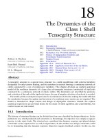
For the study and application of feedforward networks it is convenient to use in addition to
single-layer neural networks, more structured ones known as multilayer networks or

multilayer
perceptrons

. These networks with an appropriate number of hidden levels have received consider-
able attention because of better representation capabilities and the possibility of learning highly
nonlinear mappings. The typical network topology that represents a multilayer perceptron
(Figure 24.1) consists of an input layer, a sufficient number of hidden layers, and the output layer.
The following recursive relations define the network with

k

+ 1 layers:

y

0

=

u

(24.3)
(24.4)
where

y

l

is vector of neuron inputs in the

l

-layer (

y

k



=

y –

output of

k

+ 1 is the network layer,

u

is network input,

f

l

is the activation function for the

l

layer,

W

l

is the weighting matrix between
layers is the adjoint vector

y

j

. In the previous equation, bias vector is absorbed
by the weighting matrix.
yfWy l k
llll
==
−
(), ,,
1
1 K
llyy
jj
−=11 i, [ ,]

8596Ch24Frame Page 642 Tuesday, November 6, 2001 9:43 PM
© 2002 by CRC Press LLC


Each layer has an appropriate number of neural units, where each neural unit has some specific
activation function (usually a logistic sigmoid function). The weights of the networks are incre-
mentally adjusted according to appropriate learning rules, depending on the task, to improve the
system performance. They can be assigned new values in two ways: either via some prescribed
offline algorithm that remains fixed during the operation, or adjusted by a learning process. Several
powerful learning algorithms exist for feedforward networks, but the most commonly used algo-
rithm is the

backpropagation algorithm

.

9

The backpropagation algorithm as a typical supervised
learning procedure that adjusts weights in the local direction of greatest error reduction (steepest
descent gradient algorithm) using the square criterion between the real network output and desired
network output.
An RBF network approximates an input–output mapping by employing a linear combination of
radially symmetric functions. The

k –



th

output

y

k

is given by:
(24.5)
where:
(24.6)
The RBF network always has one hidden layer of computational modes with a nonmonotonic
activation function

φ

(.). Theoretical studies have shown that the choice of activation function

φ

(.)
is not very crucial to the effectiveness of the network. In most cases, the Gaussian RBF given by
(24.6) is used, where

c

i

and

σ

i

are selected centers and widths, respectively.
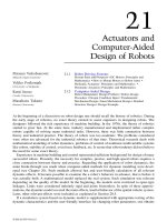
One of the earliest sensory connectionist methods capable of serving as an alternative to the
well-known backpropagation algorithm is the CMAC (cerebellar model arithmetic computer)

20

(Figure 24.2). The CMAC topology consists of a three-layer network, one layer being the sensory
or command input, the second the association layer, and the third the output layer. The association
layer is conceptual memory with high dimensionality. On the other hand, the output layer is the
actual memory with low dimensionality. The connections between these two layers are chosen in

a random way. The adjustable weights exist only between the association layer and the output layer.
Using supervised learning, the training set of patterns is presented and, accordingly, the weights
are adjusted. CMAC uses the Widrow-Hoff LMS algorithm

6

as a learning rule.

FIGURE 24.1

Multilayer perceptron.
yu w u
kki
i
i
m
() ()=
=
∑
φ
1
φφ φ σ
η
σ
( ) ( ) exp , ,uuc r r
ii ii
i
=−
()
==

()
≥≥
−
2
2
2
00

8596Ch24Frame Page 643 Tuesday, November 6, 2001 9:43 PM
© 2002 by CRC Press LLC


CMAC is an associative neural network using the feature that only a small part of the network
influences any instantaneous output. The associative property built into CMAC enables local
generalization; similar inputs produce similar outputs while distant inputs produce nearly indepen-
dent outputs. As a result, we have fast convergence properties. It is very important that practical
hardware realization using logical cell arrays exists today.
If the network possesses some cycle or loop, then it is a feedback or recurrent neural network.
In a recurrent network the system has an internal state, and the output will also depend on the
internal state of the system. These networks are essentially nonlinear dynamic systems with stability
problems. There are many different versions of inner and outer recurrent neural networks (recurrent
versions of multilayer perceptrons) for which efficient learning and stabilization algorithms must
be synthesized. One of the most commonly used recurrent networks is the Hopfield

23

type neural
network that is very suitable for optimization problems. Hopfield introduced a network that
employed a continuous nonlinear function to describe the output behavior of the neurons. The
neurons are an approximation to biological neurons in which a simplified set of important compu-

tational properties is retained. This neural network model, which consists of nonlinear graded-
response model neurons organized into networks with effectively symmetric synaptic connections,
can be easily implemented with electronic devices. The dynamics of this network is defined by the
following equation:
(24.7)
where

α

,

β

are positive constants and

I

i

is the array of desired network inputs.
A Hopfield network can be characterized by its energy function:
(24.8)
The network will seek to minimize the energy function as it evolves into an equilibrium state.
Therefore, one may design a neural network for function minimization by associating variables in
an optimization problem with variables in the energy function.

FIGURE 24.2

Structure of CMAC network.
˙

,.., ,yyfwyIin
iiiijj
j
i
=− +








+=
∑
αβ 1
EwyyIy
ij i j i i
i
n
ji
n
=− −
===
∑∑∑
1
2
111

8596Ch24Frame Page 644 Tuesday, November 6, 2001 9:43 PM

© 2002 by CRC Press LLC


ART networks

are neural networks based on the Adaptive Resonance Theory of Carpenter and
Grossberg.

17

An ART network selects its first input as the exemplar for the first cluster. The next
input is compared to the first cluster exemplar. It is clustered with the first if the distance to the
first cluster is less than a threshold. Otherwise it is the exemplar for a new cluster. This procedure
is repeated for all the following inputs. If an input is clustered with the

j

th cluster, the weights of
the network are updated according to the following formulae
(24.9)

ν

ij

(

t

+ 1) =

u

i

v

ij

(

t

) (24.10)
where

i

= 1, 2, …,

M

. ART networks belong to the class of unsupervised learning networks. They
are stable because new input patterns do not erase previously learned information. They are also
adaptive because new information can be incorporated until full capacity of the architecture is
utilized.
Proposed neural networks can be classified according to their ability to generalize. CMAC is a
local generalizing neural network, while MLPs and recurrent MLPs are suitable for global gener-
alization. RBF networks are placed between them. The choice for either one of the networks depends
on the requirement for local generalization. When a strong local generalization is needed, a CMAC

is most suitable. For global generalization, MLPs and recurrent MLPs provide a good alternative,
combined with an improved weight adjustment algorithm.

24.2.3 Learning Principles and Rules

Adaptation (or machine learning) deals with finding weights (and sometimes a network topology)
that will produce the desired behavior. Usually, the learning algorithm works from training exam-
ples, where each example incorporates correct input–output pairs (

supervised learning

). This
learning form is based on the acquisition of mapping by the presentation of training exemplars
(input–output data). Different than supervised learning,

reinforcement learning

considers the
improvement of system performances by evaluating some realized control action that is included
in the learning rules. Unsupervised learning in connectionist learning is when processing units
respond only to interesting patterns on their inputs that are based on internal learning function.
The topology of the network during the training process can be fixed or variable based on
evolution and regeneration principles.
The different iterative adaptation algorithms proposed so far are essentially designed in accor-
dance with the

minimal disturbance principle:

Adapt to reduce output error for the current training
pattern, with minimal disturbance to responses already learned. Two principal classes of algorithms

can be distinguished:

Error-correction rules,

alter the weights of a network to correct the error in the output response
to the present input pattern.

Gradient-based rules,

alter the weights of a network during each pattern presentation by a
gradient descent with the objective of reducing mean-square error, averaged over training
patterns.
The error-correction rules for networks often tend to be ad hoc. They are most often used when
training objectives are not easily quantified, or when a problem does not lend itself to tractable
analysis (for instance, networks that contain discontinuous functions, e.g., signum networks).
Gradient adaptation techniques are intended for minimization of the mean-square error associated
with an entire network of adaptive elements:
wt
vtu
vtu
ij
ij i
i
n
ij i
()
()
.()
+=
+

=
1
05
1
σ

8596Ch24Frame Page 645 Tuesday, November 6, 2001 9:43 PM
© 2002 by CRC Press LLC


(24.11)
where is the square error for particulary patterns.
The most practical and efficient algorithms typically work with one pattern presentation at a
time. This approach is referred to as

pattern learning

, as opposite to

batch learning

, in which
weights are adapted after presentation of all the training patterns (true

real-time learning

is similar
to pattern learning, but it is performed with only one pass through the data). Similar, to the single-
element case, in place of the true MSE function, the instantaneous sum squared error

e

2

(

t

) is
considered, which is the sum of the square errors at each of the

N

y

outputs of the network:
(24.12)
The corresponding instantaneous gradient is
(24.13)
where

w

(

t

) denotes a vector of all weights in the network. The steepest descent with the instanta-
neous gradient is a process presented by

w

(

t

+ 1) =

w

(

t

) +

∆

w

(

t

)
(24.14)
The most popular method for estimating the gradient is the backpropagation algorithm.
The backpropagation algorithm or generalized delta rule is the basic training algorithm for multilayer
perceptrons. The basic analysis of an algorithm application will be shown using a three-layer perceptron
(one hidden layer with a sigmoid function in the hidden and output layers). The main relations in the

training process for one input–output pair

p

=

p

(

t

) are given by the following relations:
(24.15)
(24.16)
(24.17)
(24.18)
(24.19)
where are input vectors of the hidden and output layers of the network; are output
vectors of the hidden and output layers; are weighting
factors;

w

tuij
is the weighting factor that connects neuron j in layer t with neuron i in output layer
eet
i
i
N

t
T
y
22
11
=
==
∑∑
[()]
et
i
2
()
et et
i
i
N
y
22
1
() [ ()]=
=
∑
Et
et
wt
=∇ =
∂
∂
ˆ

()
()
()
2
∆wt t() (
ˆ
())=−∇µ
ˆ
()∇ t
sWusR
ppTpp
L
21212
1
= ε
osaLo
a
p
a
pp
22120
11 1 1=+− = =/( exp( )) , , K
sWosR
ppTpp
N
y
32323
= ε
osbN
b

p
b
p
y
33
11 1=+ − =/( exp( )) , , K
yo c N
c
p
c
p
y
==
3
1 ,,K
ss
p p
23
, oo
pp
23
,
Ww tWw t
p
ij
Nu L
p
ij
LN
y

12 12
11
23 23
11
==
+×
+×
[ ( )], [ ( )]
8596Ch24Frame Page 646 Tuesday, November 6, 2001 9:43 PM
© 2002 by CRC Press LLC
u; is the input vector -number of inputs; y
p
is the output vector (N
y —
number of
outputs; L
1
= number of neurons in a hidden layer).
The square error criterion can be defined as:
(24.20)
where is the desired value of the network output; y
p
je output value of the networks; E
p
is the
value of the square criterion for one pair of input–output data; P is the set of input–output pairs.
The corresponding gradient component for the output layer is
(24.21)
(24.22)
where f

gi
is the activation function for neuron i in layer g.
For the hidden layer, the gradient component is defined by:
(24.23)
(24.24)
Based on previous equations, starting from the output layer and going back, the error backprop-
agation algorithm is synthesized. The final version of the algorithm modified by weighting factors
is defined by the following relations:
(24.25)
(24.26)
(24.27)
u
p
1
(;uN
p
u10
1=
EE yy
p
pP
pp
pP
== −
∈∈
∑∑
05
2
.
ˆ

ˆ
y
p
∂
∂
=
∂
∂
=
∂
∂
∂
=−
∈∈ ∈
∑∑ ∑
E
w
E
w
E
s
s
w
o
ij
p
ij
pP
p
i

p
i
p
ij
pP
i
p
j
p
pP
23 23 3
3
23
32
δ
δ
33333i
p
i
p
i
p
i
p
i
p
i
p
i
p

ii
p
y y df ds y y f s=− =−
′
(
ˆ
)/ (
ˆ
)()
∂
∂
=
∂
∂
=
∂
∂
∂
=
∂
∂
∂
∂
∂
∂
∂
∂
=−
′
∈∈

∈
∈
∑∑
∑∑
∑∑
E
w
E
w
E
s
s
w
E
s
s
o
o
s
s
w
wfsu
ij
p
ij
pP
p
i
p
i

p
ij
pP
p
r
p
rpP
r
p
i
p
j
p
i
p
i
p
ij
r
p
ri i i
p
j
p
rpP
12 12 2
2
12
3
3

2
2
2
2
12
3232 2 1
δ ()
=−
∈
∑
δ
21i
p
j
p
pP
u
δδ
τ232322i
pp
ri i i
p
r
wfs=
′
∑
()
δ
333iiiii
tytytfst() (

ˆ
() ()) ( ())=−
′
∆wt
E
w
to t
ij
ij
ij23
23
32
() () ()=−
∂
∂
=ηηδ
δδ
232322irriii
r
ttwtfst() () () ( ())=
′
∑
8596Ch24Frame Page 647 Tuesday, November 6, 2001 9:43 PM
© 2002 by CRC Press LLC
(24.28)
(24.29)
(24.30)
where η is the learning rate.
Also, numerous variants are used to speed up the learning process in the backpropagation
algorithm. The one important extension is the momentum technique which involves a term propor-

tional to the weight change from the previous iteration:
w(t + 1) = w(t) + ∆w(t)
(24.31)
The momentum technique serves as a low-pass filter for gradient noise and is useful in situations
when a clean gradient estimate is required, for example, when a relatively flat local region in the
mean square error surface is encountered. All gradient-based methods are subject to convergence
on local optima. The most common remedy for this is the sporadic addition of noise to the weights
or gradients, as in simulated annealing methods. Another technique is to retrain the network several
times using different random initial weights until a satisfactory solution is found. Backpropagation
adapts the weights to seek the extremum of the objective function whose domain of attraction
contains the initial weights. Therefore, both choice of the initial weights and the form of the
objective function are critical to the network performance. The initial weights are normally set to
small random values. Experimental evidence suggests choosing the initial weights in each hidden
layer in a quasi-random manner, which ensures that at each position in a layer’s input space the
outputs of all but a few of its elements will be saturated, while ensuring that each element in the
layer is unsaturated in some region of its input space.
There are more different learning rules for speeding up the convergence process of the back-
propagation algorithm. One interesting method is using recursive least square algorithms and the
extended Kalman approach instead of gradient techniques.
12
The training procedure for the RBF networks involves a few important steps:
Step 1: Group the training patterns in M subsets using some clustering algorithm (k-means
clustering algorithm) and select their centers c
i
.
Step 2: Compute the widths, σ
i
, (i = 1, …, m), using some heuristic method (p-nearest neighbor
algorithm).
Step 3: Compute the RBF activation functions φ

i
(u), for the training inputs.
Step 4: Compute the weight vectors by least squares.
24.3 Neural Network Issues in Robotics
Possible applications of neural networks in robotics include various purposes suh as vision systems,
appendage controllers for manufacturing, tactile sensing, tactile feedback gripper control, motion
control systems, situation analysis, navigation of mobile robots, solution to the inverse kinematic
problem, sensory-motor coordination, generation of limb trajectories, learning visuomotor coordi-
nation of a robot arm in 3D, etc.
5,11,16,38,39,43
All these robotic tasks can be categorized according to
the type of hierarchical control level of the robotic system, i.e., neural networks can be applied at
a strategic control level (task planning), at a tactic control level (path planning), and at an executive
∆wt
E
w
tu t
ij
ij
ij12
12
21
() () ()=−
∂
∂
=ηηδ
wt wt wt
ij ij ij23 23 23
1( ) () ()+= +∆
wt wt wt

ij ij ij12 12 12
1( ) () ()+= +∆
∆∆wt t wt() ( ) (
ˆ
()) ( )=−⋅−∇ +⋅ −11ηµ η
8596Ch24Frame Page 648 Tuesday, November 6, 2001 9:43 PM
© 2002 by CRC Press LLC
control level (path control). All these control problems at different hierarchical levels can be
formulated in terms of optimization or pattern association problems. For example, autonomous
robot path planning and stereovision for task planning can be formulated as optimization problems,
while on the other hand, sensor/motor control, voluntary movement control, and cerebellar model
articulation control can be formulated as pattern association tasks. For pattern association tasks,
neural networks in robotics can have the role of function approximation (modeling of input/output
kinematic and dynamic relations) or the role of pattern classification necessary for control purposes.
24.3.1 Kinematic Robot Learning by Neural Networks
It is well known in robotics that control is applied at the level of the robot joints, while the desired
trajectory is specified through the movement of the end-effector. Hence, a control algorithm requires
the solution of the inverse kinematic problem for a complex nonlinear system (connection between
internal and external coordinates) in real time. However, in general, the path in Cartesian space is
often very complex and the end-effector location of the arm cannot be efficiently determined before
the movement is actually made. Also, the solution of the inverse kinematic problem is not unique,
because in the case of redundant robots there may be an infinite number of solutions. The conven-
tional methods of solution in this case consist of closed-form and iterative methods. These are
either limited only to a class of simple non-redundant robots or are time-consuming and the solution
may diverge because of a bad initial guess. We refer to this method as the position-based inverse
kinematic control. The velocity-based inverse kinematic control directly controls the joint velocity
(determined by the external and internal velocities of the Jacobian matrix). Velocity-based inverse
kinematic control is also called inverse Jacobian control.
The goal of kinematic learning methods is to find or approximate two previously defined
mappings: one between the external coordinate target specified by the user and internal values of

robot coordinates (position-based inverse kinematic control) and a second mapping connected to
the inverse Jacobian of the robotic system (velocity-based inverse kinematic control).
In the area of position-based inverse kinematic control problems various methods have been
proposed to solve them. The basic idea common to all these algorithms is the use of the same
topology of the neural network (multilayer perceptron) and the same learning rule: the backprop-
agation algorithm. Although the backpropagation algorithms work for robots with a small number
of degrees of freedom, they may not perform in the same way for robots with six degrees of
freedom. In fact, the problem is that these methods are naive, i.e., in the design of neural network
topology some knowledge about kinematic robot model has not been incorporated. One solution
is to use a hybrid approach, i.e., a combination of the neural network approach with the classic
iterative procedure. The iterative method gives the final solution in joint coordinates within the
specified tolerance.
In the velocity-based kinematic approaches, the neural network has to map the external velocity
into joint velocity. A very interesting approach has been proposed using the context-sensitive
networks. It is an alternative approach to the reduction of complexity, as it proposes partition of
the network input variables into two sets. One set (context input) acts as the input to a context
network. The output of the context network is used to set up the weights of the function network.
The function network maps the second set of input variables (function input) to the output. The
original function to be learned is decomposed into a parameterized family of functions, each of
which is simpler than the original one and is thus easier to learn.
Generally, the main problem in all kinematic approaches is accurately tracking a predetermined
robot trajectory. As is known, in most kinematic connectionist approaches, the kinematic input/out-
put mapping is learned offline and then control is attempted. However, it is necessary to examine
the proposed solutions by learning control of manipulation robots in real-time, because the robots
are complex dynamic systems.
8596Ch24Frame Page 649 Tuesday, November 6, 2001 9:43 PM
© 2002 by CRC Press LLC
24.3.2 Dynamic Robot Learning at the Executive Control Level
As a solution in the context of robot dynamic learning, neural network approaches provide the
implementation tools for complex input/output relations of robot dynamics without analytic mod-

eling. Perhaps the most powerful property of neural networks in robotics is their ability to model
the whole controlled system itself. In this way the connectionist controller can compensate for a
wide range of robot uncertainties. It is important to note that the application of the connectionist
solution for robot dynamic learning is not limited only to noncontact tasks. It is also applicable to
essential contact tasks, where inverse dynamic mapping is more complex, because dependence on
contact forces is included.
The application of the connectionist approach in robot control can be divided according to the
type of learning into two main classes: neurocontrol by supervised and neurocontrol by unsupervised
learning.
For the first class of neurocontrol a teacher is assumed to be available, capable of teaching the
required control. This is a good approach in the case of a human-trained controller, because it can
be used to automate a previously human-controlled system. However, in the case of automated
linear and nonlinear teachers, the teacher’s design requires a priori knowledge of the dynamics of
the robot under control. The structure of the supervised neurocontrol involves three main compo-
nents, namely, a teacher, the trainable controller, and the robot under control.
1
The teacher can be
either a human controller or another automated controller (algorithm, knowledge-based process,
etc.). The trainable controller is a neural network appropriate for supervised learning prior to
training. Robot states are measured by specialized sensors and are sent to both the teacher and the
trainable controller. During control of the robot by the teacher, the control signals and the state
variables of the robot are sampled and stored for neural controller training. At the end of successful
training the neural network has learned the right control action and replaces the teacher in controlling
the robot.
In unsupervised neural learning control, no external teacher is available and the dynamics of the
robot under control is unknown and/or involves severe uncertainties. There are different principal
architectures for unsupervised robot learning.
In the specialized learning architecture (Figure 24.3), the neural network is tuned by the error
between the desired response and actual response of the system. Another solution, generalized
learning architecture (Figure 24.4), is proposed in which the network is first trained offline based

on control error, until good convergence properties are achieved, and then put in a real-time
feedforward controller where the network continues its adaptation to system changes according to
specialized learning procedures.
The most appropriate learning architectures for robot control are feedback-error learning archi-
tecture and adaptive learning architecture. The feedback-error learning architecture (Figure 24.5)
is an exclusively online achitecture for robot control that enables simultaneous processing of
learning and control. The primary interest is learning an inverse dynamic model of robot mechanism
for the tasks with holonomic constraints, where exact robot dynamics is generally unknown. The
neural network as part of feedforward control generates necessary driving torques in robot joints
as a nonlinear mapping of robot desired internal coordinates, velocities, and accelerations:
(24.32)
where P
i
εR
n
is a joint-driving torque generated by a neural network; are adaptive weighting
factors between neuron j in a – th layer and neuron k in b – th layer; g is nonlinear mapping.
According to the integral model of robotic systems, the decentralized control algorithm with
learning has the form

P gw qqq i n
i
jk
ab
ddd
==(,,
˙
,
˙˙
),,.1 K

w
jk
ab
8596Ch24Frame Page 650 Tuesday, November 6, 2001 9:43 PM
© 2002 by CRC Press LLC
FIGURE 24.3 Specialized learning architecture.
FIGURE 24.4 Generalized learning architecture.
FIGURE 24.5 Feedback-error learning architecture.
8596Ch24Frame Page 651 Tuesday, November 6, 2001 9:43 PM
© 2002 by CRC Press LLC
(24.33)
(24.34)
where f
i
is the nonlinear mapping which describes the nature of the robot actuator model;
KP,KF,KIεR
n×n
are position, velocity, and integral local feedback gains, respectively; εεR
n
is the
feedback error. Training and learning the proposed connectionist structure can be accomplished
using the well-known backpropagation algorithm.
9
In the process of training we can use the feedback
control signal:
(24.35)
where is the output error for the backpropagation algorithm.
A more recent and sophisticated learning architecture (adaptive learning architecture) involves
the neural estimator that identifies some robot parameters using available information from robot
sensors (Figure 24.6). Based on information from the neural estimator, the robot controller modifies

its parameters and then generates a control signal for robot actuators. The robot sensors observe
the status of the system and make available information and parameters to the estimator and robot
controller. Based on this input, the neural estimator changes its state, moving in the state space of
its variables. The state variables of the neural estimator correspond exactly to the parameters of
robot controller. Hence, the stable-state topology of this space can be designed so that the local
minima correspond to an optimal law.
The special reactive control strategy applied to robotic dynamic control
51
can be characterized
as reinforcement learning architecture. In contrast to the supervised learning paradigm, the role of
the teacher in reinforcement learning is more evaluative than instructional. The teacher provides
the learning system with an evaluation of the system performance of the robot task according to a
certain criterion. The aim of this learning system is to improve its performance by generating
appropriate outputs. In Gullapalli
51
a stochastic reinforcement learning approach with application
in robotics for learning functions with continuous outputs is presented. The learning system
computes real-valued output as some function of a random activation generated using normal
distribution. The parameters of normal distribution are the mean and the standard deviation that
FIGURE 24.6 Sensor-based learning architecture.

uu u i n
iii
ff
ii
fb
=+ =1, , .K
u fqqqP KP KD KI dti n
ii
ddd

ii i ii i ii i
=−−−=
∫
(,
˙
,
˙˙
,)
˙
,,.εε ε 1 K

eui n
i
bp
i
fb
==1, ,K
eR
i
bp
n
ε
8596Ch24Frame Page 652 Tuesday, November 6, 2001 9:43 PM
© 2002 by CRC Press LLC
depend on current input patterns. The environment evaluates the unit output in the context of input
patterns and sends a reinforcement signal to the learning system. The aim of learning is to adjust
the mean and the standard deviation to increase the probability of producing the optimal real value
for each input pattern.
A special group of dynamic connectionist approaches is the methods that use the “black-box”
approach in the design of neural network algorithms for robot dynamic control. The “black box”

approach does not use any a priori experience or knowledge about the inverse dynamic robot
model. In this case it is a multilayer neural network with a sufficient number of hidden layers. All
we need to do is feed the multilayer neural network the necessary information (desired positions,
velocities, and accelerations at the network input and desired driving torque at the network output)
and let it learn by test trajectory. In Ozaki et al.
48
a nonlinear neural compensator that incorporates
the idea of computed torque method is presented. Although the pure neural network approach
without knowledge about robot dynamics may be promising, it is important to note that this approach
will not be very practical because of the high dimensionality of input–output spaces. Bassi and
Bekey
10
use the principle of functional decomposition to simplify robot dynamics learning. This
method includes a priori knowledge about robot dynamics which, instead of being specific knowl-
edge corresponding to a certain type of robot models, incorporates common invormation about
robot dynamics. In this way, the unknown input–output mapping is decomposed into simpler
functions that are easier to learn because of smaller domains. In Kati´c and Vukobratovi´c,
12
similar
ideas in the development of the fast learning algorithm were used with decomposition at the level
of internal robot coordinates, velocities, and accelerations.
The connectionist approach is very efficient in the case of robots with flexible links or for a flexible
materials handling system by a robotic manipulators where the parameters are not exactly known and
the learning capability is important to deal with such problems. Because of the complex nonlinear
dynamical model, the recurrent neural network is very suitable for compensating flexible effects.
With recent extensive research in the area of robot position/force control, a few connectionist
learning algorithms for constrained manipulation have been proposed. We can distinguish two
essential different approaches: one, whose aim is the transfer of human manipulation skills to robot
controllers, and the other, in which the manipulation robot is examined as an independent dynamic
system in which learning is achieved through repetition of the work task.

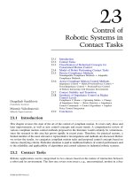
The principle of transferring human manipulation skill (Figure 24.7) has been developed in the
papers of Asada and co-workers.
18
The approach is based on the acquisition of manipulation skills
and strategies from human experts and subsequent transfer of these skills to robot controllers. It is
essentially a playback approach, where the robot tries to accomplish the working task in the same
way as an experienced worker. Various methods and techniques have been evaluated for acquisition
and transfer of human skills to robot controllers.
This approach is very interesting and important, although there are some critical issues related
to the explicit mathematical description of human manipulation skill because of the presence of
subconscious knowledge and inconsistent, contradictory, and insufficient data. These data may
cause system instability and wrong behavior by the robotic system. As is known, dynamics of the
human arm and a robot arm are essentially different, and therefore it is not possible to apply human
skill to robot controllers in the same way. The sensor system for data acquisition of human skill
can be insufficient for extracting a complete set of information necessary for transfer to robot
controllers. Also, this method is inherently an offline learning method, whereas for robot contact
tasks online learning is a very important process because of the high level of robot interaction with
the environment and unpredictable situations that were not captured in the skill acquisition process.
The second group of learning methods, based on autonomous online learning procedures with
working task repetition, have also been evaluated through several algorithms. The primary aim is
to build internal robot models with compensation of the system uncertainties or direct adjustment
of control signals or parameters (reinforcement learning). Using a combination of different intel-
ligent paradigms (fuzzy + neuro) Kiguchi and Fukuda
25
proposed a special algorithm for approach,
8596Ch24Frame Page 653 Tuesday, November 6, 2001 9:43 PM
© 2002 by CRC Press LLC
contact, and force control of robot manipulators in an unknown environment. In this case, the robot
manipulator controller, which approaches, contacts, and applies force to the environment, is
designed using fuzzy logic to realize human-like control and then modeled as a neural network to

adjust membership functions and rules to achieve the desired contact force control.
As another exposed problem in control robotic contact tasks, the connectionist approach is used
for dynamic environment identification. A new learning control concept based on neural network
classification of unknown dynamic environment models and neural network learning of robot
dynamic model has been proposed.
13
The method classifies characteristics of environments by using
multilayer perceptrons based on the first neural network, and then determines the control parameters
for compliance control using the estimated characteristics. Simultaneously, using the second neural
network, compensation of robot dynamic model uncertainties is accomplished. The classification
capability of the neural classifier is realized by an efficient offline training process. It is important
that the pattern classification process can work in an online manner as a part of selected compliance
control algorithm.
The first objective is the application of connectionist structures to fast online learning of robotic
system uncertainties as a part of the stabilizing control algorithm mentioned previously. The role
of the connectionist structure has a broader sense, because its aim is to compensate possible
uncertainties and differences between real robot dynamics and assumed dynamics defined by the
user in the process of control synthesis. Hence, to achieve good tracking performance in the presence
of model uncertainties, a fixed non-recurrent multilayer perceptron is integrated into the non-
learning control law with the desired quality of transient processing for interaction force.
In this case, compensation by neural network is connected to the uncertainties of robot dynamic
model. But, the proposed learning control algorithm does not work in a satisfactory way if there
is no sufficiently accurate information about the type and parameters of the robot environment
model. Hence, to enhance connectionist learning of the general robot-environment model, a new
method is proposed whose main idea is using a neural network approach through an offline learning
process and online sufficiently exact classification of robot dynamic environment. The neural
network classifier based on a four-layer perceptron is chosen due to good generalization properties.
Its objective is to classify the model profile and parameters of environment in an online manner.
In the acquisition process, based on real-time realization of proposed contact control algorithms
and using previously chosen sets of different working environments and model profiles of working

environments, some force data from force sensors are measured, calculated, and stored as special
input patterns for training the neural network. On the other side, the acquisition process must be
FIGURE 24.7 Transfer of human skills to robot controllers by the neural network approach.
8596Ch24Frame Page 654 Tuesday, November 6, 2001 9:43 PM
© 2002 by CRC Press LLC
accomplished using various robot environments, starting with the environment with a low level of
system characteristics (for example, with a low level of environment stiffness) and ending with an
environment with a high level of system characteristics (with high level of environment stiffness).
As another important characteristic in the acquisition process, different model profiles of the
environment are used based on additional damping and stiffness members that are added to the
basic general impedance model.
After that, during the extensive offline training process, the neural network receives a set of
input–output patterns, where the input variables form a previously collected set of force data. As
a desired output, the neural network has a value between 0 and a value defined by the environment
profile model (the whole range between 0 and 1) that exactly defines the type of training robot
environment and environment model. The aim of connectionist training is for the real output of
the neural network for given inputs to be exact or very close to the desired output value determined
for an appropriate training robot environment model.
After the offline training process with different working environments and different environment
model profiles, the neural classifier is included in the online version of the control algorithm to
produce some value at the network’s output between 0 and 1. In the case of an unknown environ-
ment, information from the neural classifier output can be utilized efficiently for calculating the
necessary environment parameters by linear interpolation procedures. Figure 24.8 shows the overall
structure of the proposed algorithm.
24.3.3 Sensor-Based Robot Learning
A completely different approach of connectionist learning uses sensory information for robot neural
control. Sensor-based control is a very efficient method in overcoming problems with robot model
and environment uncertainties, because sensor capabilities help in the adaptation proces without
explicit control intervention. It is adaptive sensor-motor coordination that uses various mappings
given by the robot sensor system. Particular attention has been paid to the problem of visuo-motor

coordination, in particular for eye–head and arm–eye systems. In general, in visuo-motor coordi-
nation by neural networks, visual images of the mechanical parts of the systems can be directly
related to posture signals. However, tactile-motor coordination differs significantly from visuo-
motor because the intrinsic dependency on the contacted surface. The direct association of tactile
sensations with positioning of the robot end-effector is not feasible in many cases, hence it is very
FIGURE 24.8 Scheme of the connectionist control law stabilizing interaction force.
8596Ch24Frame Page 655 Tuesday, November 6, 2001 9:43 PM
© 2002 by CRC Press LLC
important to understand how a given contact condition will be modified by motor actions. The task
of the neural network in these cases is to estimate the direction of a feature-enhancing motor action
on the basis of modifications in the sensed tactile perception.
After many years of being thought impractical in robot control, it was demonstrated that CMAC
could be very useful in learning state-space dependent control responses.
56
A typical demonstration
of CMAC application in robot control involves controlling an industrial robot using a video camera.
The robot’s task is to grasp an arbitrary object lying on a conveyor belt with a fixed orientation or
to avoid various obstacles in the workspace. In the learning phase, visual input signals about the
objects are processed and combined into a target map through modifiable weights that generate the
control signals for the robot’s motors. The errors between the actual motor signals and the motor
signals computed from the camera input are used to incrementally change the weights. Kuperstain
33
has presented a similar approach using the principle of sensory-motor circular reaction
(Figure 24.9). This method relies on consistency between sensory and motor signals to achieve
unsupervised learning. This learning scheme requires only availability of the manipulator, but no
formal knowledge of robotic kinematics. Opposite to previously mentioned approaches for visuo-
motor coordination, Rucci and Dario
34
experimentally verified autonomous learning of tactile-motor
coordination by a Gaussian network for a simple robotic system composed of a single finger

mounted on a robotic arm.
24.4 Fuzzy Logic Approach
24.4.1 Introduction
The basic idea of fuzzy control was conceived by L. Zadeh in his papers from 1968, 1972, and
1973.
59,61,62
The heart of his idea is describing control strategy in linguistic terms. For instance, one
possible control strategy of a single-input, single-output system can be described by a set of control
rules:
If (error is positive and error change is positive), then
control change = negative
Else if (error is positive and error change is negative), then
control change = zero
Else if (error is negative and error change is positive), then
control change = zero
Else if (error is negative and error change is negative), then
control change = positive
FIGURE 24.9 Sensory-motor circular reaction.
8596Ch24Frame Page 656 Tuesday, November 6, 2001 9:43 PM
© 2002 by CRC Press LLC