Calculation the Irreducible water saturation Swi for Nam Con Son basin from Well log data via using the Artificial neural networks
Bạn đang xem bản rút gọn của tài liệu. Xem và tải ngay bản đầy đủ của tài liệu tại đây (530.76 KB, 19 trang )
<span class='text_page_counter'>(1)</span><div class='page_container' data-page=1>
<b>C</b>
<b>alculation the I</b>
<b>rreducible water saturation Swi</b><b> for Nam Con Son basin </b>
<b>from Well log data via using the Artificial neural networks</b>
<b> </b>
<b> Đặng Song Hà</b>1<sub>, Lê Hải An</sub>2<sub>, Đỗ </sub>Minh Đức3
<i> 1. Graduate student Faculty of Geology - VNU University of Science</i>
2. Hanoi University of Mining and Geology
3. VNU University of Science
<b> Abstract: </b>
The Irreducible water saturation <i>Swi</i> is a very important parameter in oil- gas
exploration and production. Nam Con Son basin calculates<i>Swi</i> by using the Archie's
formula, is developed in four forms: Dakhnov V.H equation, Simandox equation,
Clavier equation and Schlumberger equation. To calculate<i>Swi</i>, the first have to
calculate the porosity <sub> and the volume of shale </sub><i>Vsh</i>. It is very difficult to calculate
<i>sh</i>
<i>V</i> <sub>. Therefore, the calculation of the Irreducible water saturationis </sub><i>S<sub>wi</sub></i><sub> difficult and</sub>
the accuracy is low.
This study proposes a method for calculating of the Irreducible water
saturationis <i>Swi</i> for Nam Con Son basin directly from the well log data via using the
Artificial neural networks (ANNs) without calculating the volume of shale <i>Vsh</i>
Check by using the ANN of this study to calculate <i>Swi</i>
for the wells were
calculated by other methods. Comparison results are the same. This study has
calculated <i>Swi</i>
for the wells that the Schlumberger formula can not calculate. The
results of this study revealed the new oil beds. This test demonstrates: The Artificial
neural network (ANN) model of this study is a good tool to calculate the Irreducible
water saturation <i>Swi</i>from the well log data.
<i>Keywords: ANN (Artifical neral network), the </i>Irreducible water saturation<i>Swi</i>, the
volume of shale <i>Vsh</i>, Oil and gas Potential, Nam Con Son basin
<b>1. Introduction:</b>
Nam Con Son basin, the Cenozoic clastic sediment unconformably covers up
the weathering and eroded fractured basement rocks. The oil body in the clastic
sediments has many thin beds with the different oil- water boundaries. The oil
</div>
<span class='text_page_counter'>(2)</span><div class='page_container' data-page=2>
fractured system. The oil body has the complex geological structures, is the non
traditional oil body. These specific features created serious difficulties for
investigation of the Irreducible water saturationis<i>Swi</i>
for PVEP and many foreign
contractors such as JVPC, etc…
The Nam Con Son basin currently calculates<i>Swi</i> by using the Archie's formula,
is developed in four forms: Dakhnov V.H equation, Simandox equation, Clavier
equation and Schlumberger equation [2]:
11
.
.
4
.
0
.
1
2
.
0
2
2
2
<i>sh</i>
<i>w</i>
<i>t</i>
<i>sh</i>
<i>w</i>
<i>sh</i>
<i>sh</i>
<i>sh</i>
<i>sh</i>
<i>wi</i>
<i>V</i>
<i>R</i>
<i>R</i>
<i>V</i>
<i>R</i>
<i>R</i>
<i>V</i>
<i>R</i>
<i>V</i>
<i>S</i>
In here <i>Rt</i>, <i>Rw</i>, <i>Rsh</i>
, , <i>Vsh</i> is the real resistivity of the oil reservoir, the resistivity of
the reservoir water, the resistivity of the shale, porosity, the volume of shale. To
calculate the Irreducible water saturationis <i>Swi</i>, first need to calculate the porosity
and the volume of shale <i>Vsh</i>,. The volume of shale <i>Vsh</i>, is a function [1]:
<i>Vsh</i> <i>f</i>
<i>Gr</i>
2In here:
<i>sh</i> <i>sand</i>
3<i>sand</i>
<i>Gr</i>
<i>Gr</i>
<i>Gr</i>
<i>Gr</i>
<i>Gr</i>
In
3 : <i>Gr</i><sub>, </sub><i>Grsand</i>, <i>Grsh</i> is the natural Gamma radiation intensity of the reservoir, theclean sand, clean shale, respectively. <i>Gr</i><sub> curve measured while drilling the well.</sub>
Values of <i>Grsand</i>, <i>Grsh</i> are difficult to determine accurately. The function
2 quite
complex depends on the lithology physical characteristics of the study area and is
established experimentally.
Hoang Van Quy introduced formula to calculate <i>Grsand</i>, <i>Grsh</i>, need to know the
apparent <i>Grsand</i>* ,
*
<i>sh</i>
<i>Gr</i> <sub>. Dang Song Ha suggests formula to calculate </sub><i>Gr<sub>sand</sub></i><sub>, </sub><i>Gr<sub>sh</sub></i><sub>: </sub>
.
2
)
(
.
2
)
(
<i>Gr</i>
<i>mean</i>
<i>Gr</i>
<i>Gr</i>
<i>mean</i>
<i>Gr</i>
<i>sh</i>
<i>sand</i>
4based on the basis: <i>Gr</i><sub> curve has the normal distribution (Gaussian distribution) and</sub>
the clean sand has <i>Vsh</i> 10%, the clean shale has <i>Vsh</i> 80% with <i>mean(Gr</i>)
and is
expectation and variance of the normal distribution of the <i>Gr</i><sub>curve. </sub>
Approximation of the unknowns non linear functions by the experimental
functions causes inaccuracy of the Irreducible water saturation <i>Swi</i>(will be discussed
detail in 3.7.1). In [3] Dang Song Ha offers the method of calculating the Irreducible
</div>
<span class='text_page_counter'>(3)</span><div class='page_container' data-page=3>
This study proposes a method for calculating the Irreducible water saturationis
<i>wi</i>
<i>S</i> <sub> for Nam Con Son basin directly from the well log data by using the Artificial</sub>
Neural Networks, without calculating of the volume of shale <i>Vsh</i>.
<b>2. Artifical Neural Networks (ANN)</b>
<i> ANN is the mathematical model of the biological neural network. ANN</i>
consists of 3 layers (input, hidden and output layer). The processing information of
ANN different from the algorithmic calculations. That's the parallel processing and
calculation is essentially the learning process. T<i><b>his study uses two following net. </b></i>
<i><b>2.1. Backpropagation neurall net (BPNN)</b></i>
<i> BPNN is the most commonly used net. The training set consists of a number of</i>
input signals paired with target signals. The training process consists of two steps:
the forward propagation step and the backward propagation step. The error is
calculated by comparing the outputs with the target values. BPNN uses the gradient
descent method to reduce the error. The training process creates the weight set that
can be used for calculating the water saturation <i>Swi</i>when the actual output is unknown.
<i><b>The newff function creates the BPNN network [4].</b></i>
2.2. Network with radial basis function (RBF network)
Radical basic functions is used to approximate the unknown functions based on
the input-output pairs representing the these unknown functions. The mathematical
expression of RBF is [5]:
5)
( 1
0
0
<i>N</i>
<i>i</i>
<i>i</i>
<i>i</i> <i>x</i> <i>R</i>
<i>C</i>
<i>C</i>
<i>x</i>
<i>F</i>
In here :
<i>C</i><sub>- vector containing the RBFs’ weights,</sub>
<i>R</i><sub>- vector containing the RBFs’ centers,</sub>
- the base function or the activation function of the network,
<i>F(x</i>)- function received from the output of the network,
<i>C</i>0 - deviation coefficient (possibly zero),
. <sub> - Euclidean standard.</sub>
)
<i>(x</i>
<sub>has many forms. Each form is suitable for some problems. The Gaussian function:</sub>
<sub></sub>
.
2
exp
)
(
2
<i>a</i>
<i>x</i>
<i>x</i>
</div>
<span class='text_page_counter'>(4)</span><div class='page_container' data-page=4>
RBF systems can present by the structures of the perceptron network. All
nonlinear systems can be approximated by RBF with arbitrary precision.
<i><b> The newrb function creates the RBF network [4].</b></i>
<b>3. Method </b>
Calculations <i>Swi</i> from the well log data by the Artificial neural networks (ANNs) ,
without calculating the volume of shale<i>Vsh</i> consist of the following steps: processing
data ,standardization, selection input, create training set, design and train the net,
check the accuracy of the method, and then use the net to calculate the new wells that
we call the calculating well.
<i><b>3.1. Database and selection of inputs</b></i>
Data is collected from five drilling wells: HD1, HD 2, HD3, HD4 and HD5.
The well HD1 was calculated <i>Swi</i>.We use this well to test the model. Depth of wells
from 1000m to 4500m, from 10000 to 36000 lines of data (measurement step =
0.1000m or 0.1524m). The record consists of seven curves: GR (API ) : Gamma Ray
log ; DT (.uSec/ft) : Sonic comprressional transit time; NPHI (dec): Neutron log;
RHOB (gm/cc): bulk density log; LLD (ohm.m) : laterolog deep; LLS (ohm.m ) :
laterolog shallow; MSFL (ohm.m ) : microspherically. Data of the HD3 Well:
<b>Depth GR DT NPHI RHOB LLD LLS MSFL PHI</b>
<b> (m) (api) (s/fit) (dec)(g/cm</b>3<sub>) (Ohm.m)Ohm.m)(Ohm.m) (dec)</sub>
1752.5562 99.6547 160.9300 0.4114 2.1639 2.4487 1.5846 0.1779 0.0357
1752.6562 97.5331 115.8309 0.4039 2.1709 27.8487 1.6533 0.2772 0.0535
1752.7562 98.8569 94.3495 0.3990 2.1922 1015.8776 2.2536 0.4020 0.0465
1752.8562 103.3330 94.5495 0.3964 2.2266 2883.2583 3.3394 0.5499 0.0169
………… ………… ………… ………… ………… ………… ………… ………… …………
3796.7562 54.8564 82..7477 0.1535 2.4326 4.5879.2415 3.3784 3.6821 0.1346
3796.8562 54.7599 82..3790 0.1486 2.4311 4.4730.7058 3.3323 3.7696 0.1334
3796.9562 54.4800 81..4786 0.1455 2.4392 4.3154.4286 3.2424 4.4654 0.1297
<i><b>Select inputs </b></i>
Two methods of selecting curves for inputs:
1. Select by analysing the correlation between <i>Swi</i>and the log curves:
Analysis equation (1) and equations Dakhnov VH, Simandox, Clavier. We find out:
the Irreducible water saturation <i>Swi</i>
depends on porosity (PHI curves), resistiviies <i>Rt</i>
, <i>Rw</i>, <i>Rsh</i> (LLD, LLS, MSFL curves), the volume of shale<i>Vsh</i> (GR curve). The best
curves to calculate<i>Swi</i> are GR, LLD, PHI then LLS, MSFL, NPHI, RHOB. For
</div>
<span class='text_page_counter'>(5)</span><div class='page_container' data-page=5>
00 1 2 3 4 5
5
10
15
20
25
30
GR LLD PHI RHOB MSFL
<i> Figure 1: Contribution of inputs</i>
2. Selection by ANN:
Use ANN to calculate <i>Swi</i> for the HD1 well (we call S<sub>wiANN</sub>). Schlumberger
calculated <i>Swi</i>of this well, (we call S<sub>wiBHP</sub>). Calculate the MSE between S<sub>wiANN</sub> and
SwiBHP. Call lines that <i>SwANN</i> <i>SwBHP</i> 0.03 are the non fit lines. Count the number of the
non fit lines Nnonfit from the top to the bottom of the well. The input set has MSE
smaller and Nnonfit smaller is the better input ones. By this way we remove the DT
curve. The best curves to calculate <i>Swi</i> are GR, LLD, PHI then LLS, MSFL, NPHI,
RHOB. The two selecting method match.
<i><b>Determination the number of inputs </b></i>
Input set includes 4, 5, 6 curves consist of GR, LLD, PHI and other curves. So
there is <i>C</i>414 ways to select 4 input, there is <i>C</i>426
ways to select select 5 input,
there is <i>C</i>434 ways to select 6 input.
<i><b>Detect and remove abnormal data</b></i>
The abnormal data has two types:
- Wrong record while drilling well, we call " the wrong point"
- The presence of the geological chaos: the <i>Swi</i>value varies greatly over very
short distances, this is called "the singularity point".
This study uses the Neural network to detect the abnormal points by comparing
the output values calculated by the network and the target value. If the error is greater
than the acceptable value (as we define it beforehand) the line is "the abnormal point".
The abnormal points are removed from the training set. In the calculating set,
only remove it when calculating the statistical values min (X), max (X), mean (X),
keep it when calculating the Irreducible water saturationis <i>Swi</i>.
</div>
<span class='text_page_counter'>(6)</span><div class='page_container' data-page=6>
Using BPNN we must determine the number of the hidden layers’ neurons.
Consider all 14 combinations of inputs (14 43)
2
4
1
4 <i>C</i> <i>C</i>
<i>C</i>
<sub>. Consider </sub><i>Nh</i> from 6 to 26.
Call:
<i><b> a is the regression coefficient: Output = a.target + b,</b></i>
<b> R is the training coefficient,</b>
<b> P is Performance </b>
<b>We selest if (a, R, P) satisfies: a, R nearly 1; P close to goal = 0.000500. When the</b>
input number is 4, 5 or 6 <i>Nh</i> is from 20 to 23. The best when <i>Nh</i> 22. The RBF
<b>network the newrb function defines </b><i>Nh</i> and its parameters it’self. (Limitations of
<b>newrb is only some of the nonlinear functions that the authors write.)</b>
<i><b> 3.3. Standardization of data</b></i>
In Nam Con Son basin, GR, RHOB have the Normal distribution (Gauss
distribution). NPHI has the Normal loga distribution. LLD, LLS, MSFL have the 2
distribution with many the different free degrees, dependent on the value of
mean(LLD), mean(LLS), mean(MSFL). From this survey we have the following
standardising formulas:
GR,RHOB are standardized by using the Div (X) coefficients [6] as
<i>k</i>
<i>X</i>
<i>X</i>
<i>Div</i>( ) max( )
with <i>k</i>
0.70 0.95
<sub>. </sub>Value <i>xS</i>tan<i>d</i>of <i>x</i> is:
6)
(
tan <i><sub>Div</sub></i> <i><sub>x</sub></i>
<i>x</i>
<i>x<sub>S</sub></i> <i><sub>d</sub></i>
NPHI is standardized by the exponent coefficient. Value <i>NPHIS</i>tan<i>d of NPHI is:</i>
tan 0.80. max<i>NPHI</i>
7<i>NPHI</i>
<i>d</i>
<i>s</i>
<i>e</i>
<i>e</i>
<i>NPHI</i>
LLD,LLS, MSFL are standardized by the average formula. The standardized value
<i>d</i>
<i>S</i>
<i>x</i> <sub>tan</sub>
of <i>x</i> is :
8)
(
))
(
)
(max(
*
2
)
(
2
1
)
(
)
(
*
2
tan
<i>X</i>
<i>mean</i>
<i>x</i>
<i>if</i>
<i>X</i>
<i>mean</i>
<i>X</i>
<i>X</i>
<i>mean</i>
<i>x</i>
<i>X</i>
<i>mean</i>
<i>x</i>
<i>if</i>
<i>X</i>
<i>mean</i>
<i>x</i>
<i>x<sub>S</sub></i> <i><sub>d</sub></i>
<i><b>The Matching principle</b></i>
</div>
<span class='text_page_counter'>(7)</span><div class='page_container' data-page=7>
the coefficients and parameters for the calculation well. Then we select the training set
that satisfies the matching principle (by program is named:KsatGieng.m)
<i><b>3.4. Construction the training set </b></i>
The training set consists of about 300-400 lines of data. In order to satisfy the
Matching principle, we first determine the coefficients and parameters in the
standardizasing formulas of the calculating well. To confirm the accuracy of the model,
we select well HD1 is calculated <i>Swi</i> to select the training set.
In practical application: Schlumberger calculates<i>Swi</i> for The POC. There are
many wells that Schlumberger only can calculate about 40% to 50% of the wells’
depth. We select 300-400 lines in the wells that Schlumberger calculated <i>Swi</i>
accurately
to construct the training set.The principle of selecting the training set is to examine the
calculating wells and then select the material that satisfies the Matching principle.
The input columns of the training set are sent into the LOGhl matrix, the
column <i>Swi</i> is sent into the column matrix TARGET, we have the training set
(LOGhl,TARGET), consists of 300-400 lines,
<i><b>3.5. Development of the NCS net. Training net and programming</b></i>
<i><b> </b></i>
The net calculates<i>Swi</i>for Nam Con Son basin ( call NCS net) is designed as follows:
- Input layer consists of <i>n</i> neurals: <i>x</i>1,<i>x</i>2,...<i>xn</i>,
<i>n</i>4,5,6
- Hidden layer consists of <i>Nh</i> neurals (<i>Nh</i>from 20 to 23). The transfer functions
)
<i>(x</i>
<i>f<sub>j</sub></i> <sub> with </sub> <i><sub>j</sub></i> <sub></sub><sub>1</sub><sub>,</sub><sub>2</sub><sub>...</sub><i><sub>N</sub><sub>h</sub></i> <sub> </sub>
<i> - Output layer consists of one S neural ( the Irreducible water saturation </i>.<i>Swi</i>
neural) and the transfer function <i>f</i>(<i>x</i>)tan<i>sig</i>(<i>x</i>) with <i>x</i>
0,.05,0.95
. The Irreduciblewater saturation <i>Swi</i> value of the S output neural is:
)
)
(
.
(
1 1
1
2
<i>Nh</i>
<i>j</i>
<i>n</i>
<i>i</i>
<i>i</i>
<i>ij</i>
<i>Hj</i>
<i>j</i>
<i>o</i>
<i>o</i> <i>f</i> <i>b</i> <i>f</i> <i>b</i> <i>x</i>
<i>s</i>
(9)
the transfer function <i>x</i> <i>x</i>
<i>x</i>
<i>x</i>
<i>e</i>
<i>e</i>
<i>e</i>
<i>e</i>
<i>x</i>
<i>sig</i>
<i>x</i>
<i>f</i> <sub></sub>
tan ( )
)
(
in here <i>bo</i> <sub> , </sub><i>bHj</i> are the threshold bias
of the output S neural and the <i>j</i><sub> neural of hidden layer (</sub> <i>j</i> 1,2,...<i>Nh</i><sub> )</sub>
1
<i>ij</i>
<sub> is weight of the intput neural </sub><i><sub>i</sub></i>
sent to the neural <i>j</i> of hidden layer,
2
<i>j</i>
</div>
<span class='text_page_counter'>(8)</span><div class='page_container' data-page=8>
<i>h</i>
<i>N</i> <sub> is the number of neurals of the hidden layer, </sub><i><sub>n</sub></i><sub> is the number of neurals of the</sub>
input layer. Value <i>so</i> <sub> in the training process is compared with the target value to</sub>
calculate the error. In the calculating process, it will be out. The backpropagation
algorithm presented above was used to train the net. The error is calculated by using
formula [7]:
101
1
2
<i>p</i>
<i>i</i>
<i>i</i>
<i>i</i> <i>t</i>
<i>O</i>
<i>p</i>
<i>Ero</i>
NCS net calculates <i>Swi</i> 5 input, <i>Nh</i> 22 is designed by function:
);
trainlm'
'
},
tansig'
'
tansig'
{'
1],
[22
1],
0
1;
0
1;
0
1;
0
1;
newff([0
net0
Function <i>newff</i> creates the untrained net <i>net</i>0
<i> (read: net zero)</i>
The training parameters:
net0.trainParam.epochs = 1500;
net0.trainParam.goal = 0.0005;
or: NCS newrb(LOGhl',TARGET'); <i><b>(if use Radial Basic Function) </b></i>
<i><b> Training the net is to adjust the values of the weights so that the net has the</b></i>
capable of creating the desired output response, by minimum the value of the error
function via using the gradient descent method.
At the training net: the matrix LOGhl'is sent into the input set. The information
is sent to the hidden layer, calculated, then sent to the output neural. Output neural
calculates value <i>so</i> <sub>. Matrix TARGET’ is sent into output neural. The target value is</sub>
compared with <i>so</i> <sub>to calculate the error, which determines the loop. Training net is</sub>
performed by following function:
NCS=train(net0,LOGhl',TARGET')
At the calculating net: the LOGtt' matrix (of the calculation well) is sent into
the input set. The information is passed to the hidden layer, calculated, then sent to the
output neural. The output neural calculates the output value <i>Swi</i> then this value will be
out. Calculation is performed by function:
Y=sim(NCS,LOGtt')
Program in the appendix (is called: SwNCS.m)
<i><b>3.6. Verification of the accuracy of the method</b></i>
Well HD1 we choose 10 combinations of inputs and <i>Nh</i>22. The NCS net
calculates Swi with 10 combinations of inputs. Compare SwiANN with SwiBHP. Calculate the
MSE. Results as table 1:
</div>
<span class='text_page_counter'>(9)</span><div class='page_container' data-page=9>
<b> Input</b> <sub> </sub><i>Nh</i> <b> A</b> <b> R</b> <b> P</b> <b> MSE</b>
<b>G N D P</b>
<b>G R D P</b>
<b>G D S P</b>
<b>G D M P</b>
22
22
22
22
0.98
0.99
0.99
0.99
0.99102
0.99347
0.98908
0.99254
0.00067888
0.00083185
0.00061399
0.00071675
0.000653
0.000986
0.000125
0.000664
<b>G N D S P</b>
<b>G N D M P</b>
<b>G R D M P</b>
<b>G D S M P</b>
22
22
22
22
0.98
0.99
0.98
0.99
0.99298
0.99339
0.99312
0.99271
0.00064159
0.0004999
0.00056442
0.00058316
0.000743
0.000219
0.000547
0.000386
<b>G N R D S P</b>
<b>G N R D M P</b>
22
22
0.99
0.99
0.99344
0.99339
0.0004999
0.0005649
0.000480
0.000379
<i>Table 1: 10 combinations of inputs were choosed to caoculate S</i>wi.
Compare we see the results of 10 ways to calculate this overlap. Just 4 and / or 5 inputs
are sufficient.
<i>Figure 2 shows SwiBHP</i> and SwiANN from the top to the bottom of the well. (Blue color
is ploted after, so blue color coveres red one)
0 50 100 150 200
0
0.2
0.4
0.6
0.8
1
from line 1 to line 200
S
W
0 50 100 150 200
0
0.2
0.4
0.6
0.8
1
from line 201 to line 400
S
W
0 50 100 150 200
0.2
0.4
0.6
0.8
1
from line 401 to line 600
S
W
0 50 100 150 200
0
0.2
0.4
0.6
0.8
1
from line 601 to line 800
S
W
0 50 100 150 200
0
0.2
0.4
0.6
0.8
1
from line 801 to line 1000
S
W
0 50 100 150 200
0.2
0.4
0.6
0.8
1
from line 1001 to line 1200
S
</div>
<span class='text_page_counter'>(10)</span><div class='page_container' data-page=10>
0 50 100 150 200
0
0.2
0.4
0.6
0.8
1
from line 1201 to line 1400
S
W
0 50 100 150 200
0
0.2
0.4
0.6
0.8
1
from line 1401 to line 1600
S
W
0 50 100 150 200
0
0.2
0.4
0.6
0.8
1
from line 1601 to line 1800
S
W
0 50 100 150 200
0
0.2
0.4
0.6
0.8
1
from line 1801 to line 2000
S
W
0 50 100 150 200
0
0.2
0.4
0.6
0.8
1
from line 2001 to line 2200
S
W
0 50 100 150 200
0
0.2
0.4
0.6
0.8
1
from line 2201 to line 2400
S
W
<b> Figure 2 </b>: The Irreducible water saturation Swi from the top to the bottom of the well
(Red is SwiBHP, blue is SwiANN)
Oil bodies in the clastic sediments has many thin beds from several meters to
several dozen meters [1]. To detect oil beds we group each layer 40 lines (equivalent to
6m thickness) into one point. Figure 3 below shows four calculation ways: 4 input, 5
input, 6 input and an average of 4,.5,6 iput. The same result: There are 6 oil beds
16000 1800 2000 2200 2400 2600 2800
0.2
0.4
0.6
0.8
Oil bed
Oil bed
Oil bed
Oil bed
Oil bed Oil bed
Dictribution of Sw in depth (Red is SWpoc, blue is SWann)
Depth (m), * is the central depth of the layer. (4 input)
W
a
te
r
s
a
tu
ra
ti
o
n
(
d
e
c
)
16000 1800 2000 2200 2400 2600 2800
0.2
0.4
0.6
0.8
Oil bed
Oil bed
Oil bed
Oil bed
Oil bed Oil bed
Depth (m), * is the central depth of the layer. (5 input)
</div>
<span class='text_page_counter'>(11)</span><div class='page_container' data-page=11>
16000 1800 2000 2200 2400 2600 2800
0.2
0.4
0.6
0.8
Oil bed
Oil bed
Oil bed
Oil bed
Oil bed Oil bed
Depth (m), * is the central depth of the layer.(6 input)
W
a
te
r
s
a
tu
ra
ti
o
n
(
d
e
c
)
16000 1800 2000 2200 2400 2600 2800
0.2
0.4
0.6
0.8
Oil bed
Oil bed
Oil bed
Oil bed
Oil bed Oil bed
Depth (m), * is the central depth of the layer.(4.5.6input)
W
a
te
r
s
a
tu
ra
ti
o
n
(
d
e
c
)
<i>Figure 3 : </i>The Irreducible water saturation Swi of the layers (Red is SwiBHP, blue is SwiANN, )
<b>3.7 Application</b>
<i><b>3.7.1 Limitations of the Schlumberger equation</b></i>
<b> Rewrite the Schlumberger equation:</b>
<sub></sub>
<sub></sub>
<sub> </sub>
'2
2
2
2
1
.
1
2
.
0
.
1
.
.
4
.
0
<i>T</i>
<i>R</i>
<i>V</i>
<i>R</i>
<i>R</i>
<i>V</i>
<i>R</i>
<i>V</i>
<i>V</i>
<i>R</i>
<i>S</i> <i>sh</i> <i>w</i> <i>sh</i> <i>t</i>
<i>sh</i>
<i>sh</i>
<i>sh</i>
<i>sh</i>
<i>w</i>
<i>wi</i>
Use the Lopitan rule to find the limit of the form 0
0
we have:
11.
lim
0
<i>sh</i>
<i>t</i>
<i>sh</i>
<i>wi</i>
<i>V</i>
<i>R</i>
<i>R</i>
<i>S</i>
0,1
<i>wi</i>
<i>S</i> <sub> , </sub>
0,1 <sub> và </sub><i>V<sub>sh</sub></i>
0,1 <sub>But in the sands beds contain oil- gas we have</sub>
0,0.5
<sub> and </sub><i>V<sub>sh</sub></i>
0.1, 0.5
<sub>. Since </sub><i>R<sub>sh</sub></i>2and
11 we see in the region that the realresistivity <i>Rt</i>
</div>
<span class='text_page_counter'>(12)</span><div class='page_container' data-page=12>
bottom of the well, and using the statistical probability formulas, we can calculate the
quantity <i>Swi</i> 1 of the Schlumberger formula.
Schlumberger calculates <sub> and </sub><i>Swi</i>for the POC. When calculating wrong 0
will assign 0.0001. The wrong <i>Swi</i> 0 is assigned <i>Swi</i> 0.001. The wrong <i>Swi</i> 1 is
assigned <i>Swi</i> 1.
Surveying a well Schlumberger calculated 14667 values has 894 wrong values
have to assign 0.0001 equal 6.1%. This well has 7941 values <i>Swi</i> 1 and 6723
values <i>Swi</i> 1, there are 562 wrong values <i>Swi</i> 0 have to assign are 0.001 equal
8,361%. To determine the wrong rate <i>Swi</i> 1, this study counts the lines that S<sub>wiBHP</sub> =1
but SwiANN <0.8. The number of counts matches the number, calculated from the formula
1' <sub>. </sub><sub>Thus: The above equations only give the correct value when </sub><i>S<sub>wi</sub></i>
0.15,0.70
<sub> and</sub>10
.
0
<sub>. If </sub><i>S<sub>wi</sub></i> 0.15<sub> the Schlumberger value usually is smaller than the actual value, if</sub>
70
.
0
<i>wi</i>
<i>S</i> <sub> the Schlumberger values oftens greater than the actual value. In the</sub>
Cenozoic clastic sediment there are the oil beds that .<i>Swi</i> 0.70 (specially in claystone).
So assignment <i>Swi</i> 1
can be confused, not detect these oil beds.
<i><b> 3.7.2 Application </b></i>
This study calculates <i>Swi</i>
for the segments that Schlumberger can not calculate
and / or calculate wrongly have to assign<i>Swi</i> 1. Calculations for well HD3 are
presented below. The result of this study: Discover a limestone oil bed that
<b>Schlumberger can not detect. </b>
The oil and gas reserves is calculated according to the volume formula:
<i>Q</i><i>S</i>.<i>H</i>..<i>So</i>..<i>d</i><i>K</i>..
1<i>Swi</i>
12(<i>S</i>.=area cotains oil, <i>H</i>: thickness, : conversion coefficient; <i>d</i>: oil density)
with <i>K</i> <i>S</i>.<i>H</i>. .<i>d</i> . So the oil and gas Potential is <i>Po</i><i>k</i>..
1<i>Swi</i>
. We select <i>k</i> 10, The HD3 well is drilled quite deep. From the top to the bottom of the well is
2952,43m:
Strt = 725.4809m;
Stop = 3676.0975m,
Recorded 19372 lines of data.
Schlumberger calculated <sub> and </sub><i>Swi</i>. The resulting as follows:
Can not calculate : 1747 lines = 9.02%.
</div>
<span class='text_page_counter'>(13)</span><div class='page_container' data-page=13>
Number of lines can not calculate <i>Swi</i>
= 3232 lines.
This study uses ANN to calculate <sub> and </sub><i>Swi</i>
for the whole well (Calculate
porosity <sub> of this study in [6] ). Estimate the error and look at figure 5a and 5b, We</sub>
see that the result of calculating by ANN is more accurate than by Schlumberger
method.
500 1000 1500 2000 2500 3000 3500 4000
-0.2
0
0.2
0.4
0.6
Porosity from the top to bottom of the well (Red is BHP, blue is ANN)
Depth( (m), )
P
o
ro
s
it
y
(
d
e
c
)
POC gan Phi=0.19
500 1000 1500 2000 2500 3000 3500 4000
0
0.5
1
1.5
Oil & gas saturation from top to bottom of the well (Red is BHP Blue is ANN)
Depth( (m), )
O
il
&
g
a
s
S
a
tu
(
d
e
c
)
<i> Figure 5a : Porosity from the top to the bottom of the Well.</i>
<i> 5b : Oil and gas saturation from the top to the bottom of the Well</i>
Calculate the oil- gas Potential <i>Po</i>10..
1<i>Swi</i>
: The total oil- gas Potential of BHP = 1978.719
The total oil- gas Potential of ANN = 2806.175
</div>
<span class='text_page_counter'>(14)</span><div class='page_container' data-page=14>
500 1000 1500 2000 2500 3000 3500 4000
0
0.5
1
1.5
Oil & gas Potential from the top to bottom of the well (Red is BHP, blue is ANN)
Depth( (m), )
P
o
te
n
ti
a
l
(d
e
c
)
500 1000 1500 2000 2500 3000 3500 4000
0
0.5
1
Depth( (m), )
P
o
te
n
ti
a
l
(d
e
c
)
500 1000 1500 2000 2500 3000 3500 4000
0
0.5
1
1.5
Depth( (m), )
P
o
te
n
ti
a
l(
d
e
c
)
<i> Figure 6 : </i>Oil &gas Potential of the well (Red is BHP, blue is ANN)
<b>4. Discussion:</b>
1. This study calculates<i>Swi</i> with the actual accepted accuracy without
calculating the volume of shale <i>Vsh</i> and has built up the program system (MATLAB
language) and provides the processing procedures for the calculation <i>Swi</i>problem.
2. The calculation <i>Swi</i> of this study should not be considered separately, but it
should compare the results of calculating <i>Swi</i> of this study with the results of seismic
interpretation, analysing the stratigraphic column of the drilling wells, the porosity .
Method calculates<i>Swi</i> by ANN of this study is acceptable because it is consistent with
reality, consistent with the result of seismic interpretation.
3. The ANN of this study for calculating<i>Swi</i>has the great precision because:
- Select the appropriate input set. Evaluate acurately the contribution of each
input.Three important curves for calculating <i>Swi</i>(GR, PHI, LLD) are completed before
calculating<i>Swi</i>. Correction and supplementation of GR curve is presented in [8];
calculating porosity is presented in [6]. The LLD curve is processed by the average
formula (8).
- Has built the training set to ensure the representativeness and completeness,
suitable for each calculating well. With 300-400 trainning units, the net is trained all
parameters to achieve the best.
</div>
<span class='text_page_counter'>(15)</span><div class='page_container' data-page=15>
very heterogeneous environment of Nam Con Son basin, especially the mean value
formula (8). Find out the matching principle and comply this principle strictly.
<b>5. Conclusion </b>
1. ANN is a good tool for calculating <i>Swi</i>. The best is 5 inputs, include GR,
LLD, PHI and 2 curves selecte in NPHI, RHOB, MSFL.
2. The training set should select from 300 to 400 as well. Do not choose more.
3. ANN can be used to calculate <i>Swi</i> and other parameters in the basic research
and in the actual calculations in order to build the mining production technology
diagrams.
4. The sediment basins in Vietnam are the very heterogeneous environment. So
calculating by ANN are more accurate than by the traditional methods. Because of
the approximation of the complex nonlinear function by the empirical formula is not
exact, while ANN can model any nonlinear system with arbitrary precision.
Development ANN is the right direction of research.
5. Clarify the nature of the environment of Nam Con Son basin and the
correlation of the well log data, have good knowledge of the ANN to make the right
decision: Select the network, select the activation function, select the inputs, find out
the correct standardising formulas, building the training set is important factor
<b>6. Acknowledgment </b>
The authors would like to thank: JVPC has used the results of this study to
develop the mining production technology diagrams.
<b>7. References </b>
[1] Hoàng văn Quý PVEP 2014. Ho Chi Minh city.
<i> Lecture interpretation theory well log data (in Vietnamese) </i>
[2] Lê Hải An 2012. Hanoi university of mining and geology
<i> Log Interpretation (in Vietnamese) </i>
[3] Đặng Song Hà
Calculation the Irreducible water saturation <i>Swi</i>
and determination Capillary
pressure curve Pc from Well log data
<i> VNU, Jurnal of Earth and Environmental Sciences Vol 28, No.3,2012, p 173-180</i>
<i>[4] Pof. S. Sengupta Departmen of Electionl Communication Engineering IIT</i>
</div>
<span class='text_page_counter'>(16)</span><div class='page_container' data-page=16>
[5] Bùi Công Cường: Mathematical Institute of Vietnam.
Publishing scientific and technical 2006.
<i> Artificial Neural Networks and fuzzy systems (in Vietnamese) </i>
[6] Đặng Song Hà, Lê Hải An
Determination of the porosity for the sedimentary clastic and the magmatic basement
rocks of Cuulong basin from well log data via using the artificial neural networks
<i> Hanoi university of mining and geology, Jurnal of mining and Earth Sciences</i>
<i>No.1, Vol 60, 2017,</i>
<i> [7] Girish Kumar Jha I A.R.I NewDelhi-110012 </i>
Artifical Neuralnetworks and its applications
[8] Đặng Song Hà, Lê Hải An, Đỗ Minh Đức
Correction and supplementation of the well log curves for Cuu Long oil basin by
using the Artificial Neural Networks
<i>VNU, Jurnal of Earth and Environmental Sciences</i> Vol 30, No.1,2017
<b>8. Appendix</b>
<b> Perform after preprocessing data</b>
<b> Program ’SwNCS.m’; function ‘Choa.m’. Scripts are simple.</b>
SwNCS.m
disp('Calculate the Irreducible water saturation by program SwNCS.m ');
% Data File: D:\HLDH1.doc D:\DH1.doc;
% Function Choa; Scripts : ChínhSw, tEro, InKqua, HthiKhuc, HtVia
c1=1;
c2=3;
c3= 4;
c4=5;
c5=8;
co=40;
</div>
<span class='text_page_counter'>(17)</span><div class='page_container' data-page=17>
HL= Choa(L); % Standardize the training set
L=load('D:\DH1.doc'); [n m]=size(L); disp(['Number calculate = ' num2str(n)]);
TT= Choa(L); % Standardize the calculating set
LOGhl=[HL(:,c1) HL(:,c2) HL(:,c3) HL(:,c4) HL(:,c5) ]; TARGET=HL(:,9);
LOGtt=[TT(:,c1) TT(:,c2) TT(:,c3) TT(:,c4) TT(:,c5) ];
%Create net, training NCS net
net0 = newff([ 0 1; 0 1; 0 1; 0 1; 0 1],[22 1],{'tansig''tansig'},'trainlm');
y=sim(net0,LOGhl');
net0.trainParam.epochs = 1500;
net0.trainParam.goal = 0.0005;
DH1=train(net0,LOGhl',TARGET')
Y=sim(DH1,LOGtt'); SWann=Y'; ChinhSw; % Calculate Sw by NCS net
tEro; % Calculate Ero
In= [STT Depth SWcu SWann]; Fname='D:\SwDH1.doc';
InKqua; % Print results in file :’D:\SwDH1.doc’:
XXcu= SWcu; XXann= SWann;
kh=200; HthiKhuc; vi= 40; HtVia; % Displate in Screen
disp('Finish, Continue ?' );
function [C]=Choa(L)
[n m]=size(L);
STT=L(:,1);
Depth=L(:,2);
GR=L(:,3);
NPHI=L(:,4);
RHOB=L(:,5);
LLD=L(:,6);
LLS=L(:,7);
PHI=L(:,8);
SW=L(:,9);
A=[GR NPHI RHOB LLD LLS PHI SW Depth STT];
CGR=A(:,1); CGR=CGR/180;
CNPHI =A(:,2); hs=0.8/exp(max(CNPHI)); CNPHI= hs*exp(CNPHI);
</div>
<span class='text_page_counter'>(18)</span><div class='page_container' data-page=18>
CLLD =A(:,4);
for i=1:n
x=CLLD(i);
if (x<110)
CLLD(i)=x/220;
else
CLLD(i)=1/2+ ((x-110))/3200;
end
end
LLS =A(:,5);
for i=1:n
x=CLLS(i);
if (x<40)
CLLS(i)=x/80;
else
CLLS(i)=1/2+ ((x-40))/2400;
end
end
CPHI = A(:,6); CPHI = CPHI*4;
CSW = A(:,7);
C=[CGR CNPHI CRHOB CLLD CLLS CPHI CSW Depth STT];
<b> </b>
<b> Tính độ bão hòa nước dư từ tài liệu địavật lý giếng khoan</b>
<b> bằng mạng Nơron nhân tạo cho bể Nam Côn Sơn </b>
Đặng Song Hà1<sub>, Lê Hải An </sub>2<sub> , Đỗ Minh Đức</sub>3<sub>,</sub>
1. NCS Khoa Địa chất Đại học Khoa học Tự nhiên-ĐHQGHN
2. Đại học Mỏ Địa chất
3. Đại học Khoa học Tự nhiên-ĐHQGHN
<b>Tóm tắt </b>
Độ bão hòa nươc dư ( Irreducible water saturation) <i>Swi</i> là tham số rất quan trọng
trong nghiên cứu thăm dị khai thác dầu khí. Hiện nay bể Nam Cơn Sơn tính <i>Swi</i> theo
cơng thức Archie được phát triển thành 4 dạng : Phương trình Dakhnov V.H, phương
</div>
<span class='text_page_counter'>(19)</span><div class='page_container' data-page=19>
hết phải tính độ rỗng và hàm lượng sét<i>Vsh</i>. Rất khó tính<i>Vsh</i>. Vì vậy tính<i>Swi</i>
rất khó và
độ chính xác thấp.
Nghiên cứu này đưa ra phương pháp tính<i>Swi</i><b> cho bể Nam Côn Sơn trực tiếp từ</b>
các đường cong địa vật lý giếng khoan bằng mạng nơron nhân tạo (ANN) khơng cần
tính hàm lượng sét <i>Vsh</i>.
Kiểm tra bằng cách dùng ANN của nghiên cứu này tính<i>Swi</i>cho những giếng đã
tính được <i>Swi</i>
bằng phương pháp khác. So sánh kết quả ta thấy trùng nhau. Nghiên cứu
này đã tính <i>Swi</i>
cho những giếng mà cơng thức Schlumberger khơng tính được<i>Swi</i>. Kết
quả tính của nghiên cứu này đã phát hiện ra vỉa dầu mới. Kiểm tra này chứng tỏ : Mơ
hình mạng Nơron nhân tạo (ANN) của nghiên cứu này là cơng cụ tốt để tính<i>Swi</i>từ tài
liệu ĐVLGK.
<i>Từ khóa:</i>Mạng Nơron nhân tạo(ANN), Độ bãohòa nước dư (Irreducible water saturation)
<i>wi</i>
<i>S</i>
. <sub>, Hàm lượng sét </sub>.<i>V<sub>sh</sub></i><sub>, Tiềm năng dầu khí (Oil and gas Potential), bể Nam Cơn Sơn. </sub>
<b> </b>
<b> ĐẶNG SONG HÀ </b>
</div>
<!--links-->