Modeling and simulation of wireless communication networks of VNU-IS.

<span class='text_page_counter'>(1)</span><div class='page_container' data-page=1>

analyzing Monte Carlo for evaluating research stages, they have concluded that one
can achieve long-term strategy by combining moving average crossover strategy with
CANSLIM method of William Oneil (Iavnov & Beyoglu, 2008)”.

(Mehdi Majafi, Farshid Asgari,Using CANSLIM Analysis for Evaluating Stocks of the
Companies Admitted in Tehran Stock Exchange, Journal of American Science 2013).

<b>Modeling and simulation of </b>

<b>wireless communication networks of VNU-IS.</b>

Group sciences: Trần Hoàng Anh
Nguyễn Văn Sơn
Nguyễn Văn Dũng
Lê Tự Quốc Thắng
Class: MIS2015A

</div>
<span class='text_page_counter'>(2)</span><div class='page_container' data-page=2>

<b>CHAPTER 1: INTRODUCTION TO WIRELESS LAN</b>
<b>1.1 Introduction[1]</b>

</div>
<span class='text_page_counter'>(3)</span><div class='page_container' data-page=3>

from the current set of modulation schemes in order to optimise frame transmission. In
this way, wireless devices can link rate adapt according to the channel conditions.
802.11 has not been without its problems, especially with regard to security. WLANs
are particularly vulnerable to eavesdropping, unauthorised access and denial of service
due to their broadcast nature. The original 802.11 standard had no security provisions
at all, neither authentication, encryption or data integrity. Some access-point vendors
offered authentication of the client’s physical address. The standard was amended in
1999 to support a basic protection mechanism. Wired equivalent privacy (WEP) used
cryptographic methods for authentication and encryption. The security flaws in WEP,
however, have given rise to a complete research field. In 2001, Fluhrer, Mantin, and
Shamir showed that the WEP key could be obtained within a couple hours with just a

consumer computer[2]. The authors highlighted a weakness in RC4’s key scheduling
algorithm and showed that it was possible to derive the key merely by collecting
encrypted frames and analysing them. Sincethen, more sophisticated WEP attacks have
been developed. Along with advances in computing power, the WEP key can be
recovered in seconds. A further vulnerability with WEP is that the pre-shared key is
common to all users on the same SSID. Any user associated with an SSID, therefore,
can decrypt packets of other users on the same SSID. These problems have largely
been resolved with the deprecation of WEP and the introduction of enhanced security
methods. As with the introduction of new modulation techniques, interoperability is an
issue. The current security methods rely on modern cryptography techniques which are
only available on new devices. On legacy devices, interim solutions have been
adopted.

<b>1.2 I EEE 802 Standard [2]</b>

</div>
<span class='text_page_counter'>(4)</span><div class='page_container' data-page=4>

physical channel. It implements various forms of error control, flow control and
synchronisation. In the 802 reference model, the data link layer comprises two
sub-layers, the logical link control (LLC) sub-layer and the medium access control (MAC)
sub-layer.

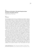
<b>Figure 1.1: shows the 802 reference model [3]</b>
Data link layer Logical link control (LLC)

</div>
<span class='text_page_counter'>(5)</span><div class='page_container' data-page=5>

<b>Figure 1.2: Wireless LANs</b>

<b>Number</b> <b>Standard</b> <b>Comment</b>

802.1 Bridging

802.2 Logical link control

( LLC )

802.3 CSMA/CD Enthernet-like

802.4 Token bus Dishanded

802.5 Token Ring Inactive

802.11 Wireless LANs Wi – FI

802.15 Wireless PANs Bluetooth and Zigbee

802.16 Wireless MANs WiMAX

LLC is defined in the IEEE 802.2 standard. Its primary function is to provide an
interface between the MAC layer and the higher layers (network layer). It performs
multiplexing functions in order to support multiple upper layer protocols. Furthermore,
it is responsible for flow control and error control. Both connectionless and
connection-orientated frame delivery schemes are supported. LLC is unconcerned with
the specific details of the LAN medium itself. That is the responsibility of the MAC
sub-layer which is primarily concerned with managing access to the physical channel.
The physical layer of 802 is responsible for the transmission and reception of bits,
encoding and decoding of signals and synchronisation (preamble processing). The
physical layer hides the specifics of the medium from the MAC sub-layer. The first 802
standards were wired LANs. Carrier sense multiple access with collision detect
(CSMA/CD) based LANs (802.3) are the most widely used. Token bus (802.4), token
ring (802.5) and fibre distributed data interface (FDDI) were also defined. Wireless
network standards emerged in the 1990s. IEEE 802.11 defined a wireless LAN
technology that operates in license free bands. 802.11 is commonly referred to as
Wi-Fi. 802.11 employs a CSMA protocol similar to 802.3 (and Ethernet). However,

instead of using collision detection, it uses collision avoidance. Wireless personal area
networks (PANs) are covered by 802.15, where 802.15.1
specifiestheBluetoothstandardand802.15.4 defines Zigbee.IEEE802.16isawireless
metropolitan area network (MAN) also known as WiMAX. Table 1.1 shows a
summary of some of the 802 standards.

</div>
<span class='text_page_counter'>(6)</span><div class='page_container' data-page=6>

The IEEE 802.11 was formed in July 1990 to develop CSMA/CA, a variation of
CSMA/CD (Ethernet)−based wireless LANs. The working group produced the first
802.11 standard in 1997, which specifies wireless LAN devices capable of operating
up to 2 Mbps using the unlicensed 2.4−GHz band. Currently, the working group has
nine basic task groups and each is identified by a letter from a to i. Following are the
current 802.11 task groups and their primary responsibilities:

 802.11a. Provides a 5−GHz band standard for 54−Mbps transmission rate.
 802.11b. Specifies a 2.4−GHz band standard for up to 11−Mbps transmission

rate.

 802.11c. Gives the required 802.11−specific information to the ISO/IEC
10038 (IEEE 802.1D) standard. • 802.11d. Adds the requirements and
definitions necessary to allow 802.11 wireless LAN equipment to operate in
markets not served by the current 802.11 standard.

 802.11e. Expands support for LAN applications with Quality of Service
requirements.• 802.11f. Specifies the necessary information that needs to be
exchanged between access points to support the P802.11 DS functions.

 802.11g. Develops a new PHY extension to enhance the performance and the
possible applications of the 802.11b compatible networks by increasing the
data rate achievable by such devices.

 802.11h. Enhances the current 802.11 MAC and 802.11a PHY with network
management and control extensions for spectrum and transmit power
management in 5−GHz license exempt bands.

 802.11i. Enhances the current 802.11 MAC to provide improvements in
security

<i><b>1.2.2 The 802.11 Standard Details [4]</b></i>

The 802.11 standard specifies wireless LANs that provide up to 2 Mbps of
transmission speed and operate in the 2.4−GHz Industrial, Scientific, and Medical
(ISM) band using either frequency−hopping spread spectrum (FHSS) or
direct−sequence spread spectrum (DSSS)[5]. The IEEE approved this standard in
1997. The standard defines a physical layer (PHY), a medium access control (MAC)
layer, the security primitives, and the basic operation modes.

</div>
<span class='text_page_counter'>(7)</span><div class='page_container' data-page=7>

The 802.11 standard supports both radio frequency− and infrared−based
physical network interfaces. However, most implementations of 802.11 use radio
frequency, and we only discuss the radio frequency−based physical interface here.
<i>802.11 Frequency Bandwidth</i>

802.11 standard−compliant devices operate in the unlicensed 2.4−GHz ISM
band. Due to the limited bandwidth available when the electromagnetic spectrum is
used for data transmission, many factors have to be considered for reliable, safe, and
high−performance operation. These factors include the technologies used to propagate
signals within the RF band, the time that a single device is allowed to have an
exclusive transmission right, and the modulation scheme. For these reasons, FCC
regulations require that radio frequency systems must use spread spectrum technology
when operating in the unlicensed bands.

<i>Spread Spectrum Technology</i>

The 802.11 standard mandates using either DSSS or FHSS. In FHSS, the radio
signal hops within the transmission band. Because the signal does not stay in one place
on the band, FHSS can elude and resist radio interference. DSSS avoids interference
by configuring the spreading function in the receiver to concentrate the desired signal,
and to spread out and dilute any interfering signal.

<i>Direct−Sequence Spread Spectrum (DSSS)</i>

In DSSS the transmission signal is spread over an allowed band. The data is
transmitted by first modulating a binary string called spreading code. A random binary
string is used to modulate the transmitted signal. This random string is called the
spreading code. The data bits are mapped to a pattern of "chips" and mapped back into
a bit at the destination. The number of chips that represent a bit is the spreading ratio.
The higher the spreading ratio, the more the signal is resistant to interference. The
lower the spreading ratio, the more bandwidth is available to the user. The FCC
mandates that the spreading ratio must be more than 10. Most products have a
spreading ratio of less than 20. The transmitter and the receiver must be synchronized
with the same spreading code. Recovery is faster in DSSS systems because of the
ability to spread the signal over a wider band.

</div>
<span class='text_page_counter'>(8)</span><div class='page_container' data-page=8>

This spread spectrum technique divides the band into smaller subchannels of
usually 1 MHz. The transmitter then hops between the subchannels sending out short
bursts of data for a given time. The maximum amount of time that a transmitter spends
in a subchannel is called the dwell time. In order for FHSS to work correctly, both
communicating ends must be synchronized (that is, both sides must use the same
hopping pattern), otherwise they lose the data. FHSS is more resistant to interference
because of its hopping nature. The FCC mandates that the band must be split into at

least 75 subchannels and that no subchannel is occupied for more than 400
milliseconds. Debate is always ongoing about the security that this hopping feature
provides. Since there are only 75 subchannels available, the hopping pattern has to be
repeated once all the 75 subchannels have been hopped. HomeRF FHSS
implementations select the initial hopping sequence in a pseudorandom fashion from
among a list of 75 channels without replacement. After the initial 75 hops, the entire
sequence is repeated without any replacement or change in the hopping order. An
intruder could possibly compromise the system by monitoring and recording the
hopping sequence and then waiting till the whole sequence is repeated. Once the
hacker confirms the hopping pattern, he or she can predict the next subchannel that
hopping pattern will be using thereby defeating the hopping advantage altogether.
HomeRF radios, for example, hop through each of the 75 hopping channels at a rate of
50 hops per second in a total of 1.5 seconds, repeating the same pattern each time,
enabling a hacker to guess the hopping sequence in 3 seconds. Nevertheless, this
technique still provides a high level of security in that expensive equipment is needed
to break it. Many FHSS LANs can be colocated if an orthogonal hopping sequence is
used. Since the subchannels in FHSS are smaller than DSSS, the number of colocated
LANs can be greater with FHSS systems. The most commonly used standard based on
FHSS is HomeRF.

<i>The MAC Layer</i>

</div>
<span class='text_page_counter'>(9)</span><div class='page_container' data-page=9>

when it is expected to receive data. The channel access mechanism is the core of the
MAC protocol. With most wired LAN using the Carrier Sense Multiple Access with
Collision Detection (CSMA/CD) it was a logical choice for the 802.11 Working Group
to apply the CSMA/CD technology when developing the MAC layer for the 802.11
standard.

The working group chose the Carrier Sense Multiple Access with Collision
Avoidance (CSMA/CA), a derivative of CSMA/CD, as the MAC protocol for the

802.11 standard. CSMA/CA works as follows: The station listens before it sends. If
someone is already transmitting, it waits for a random period and tries again. If no one
is transmitting, then it sends a short message. This message is called the
ready−to−send message (RTS). This message contains the destination address and the
duration of the transmission. Other stations now know that they must wait that long
before they can transmit. The destination then sends a short message, which is the
clear−to−send message (CTS). This message tells the source that it can send without
fear of collisions. Upon successful reception of a packet, the receiving end transmits
an acknowledgment packet (ACK). Each packet is acknowledged. If an
acknowledgment is not received, the MAC layer retransmits the data. This entire
sequence is called the four−way handshake.

<i><b>1.2.3 802.11 Security [4]</b></i>

IEEE 802.11 provides two types of data security authentication and privacy.
Authentication is the means by which one station verifies the identity of another
station in a given coverage area. In the infrastructure mode, authentication is
established between an AP and each station. When providing privacy, a wireless LAN
system guarantees that data is encrypted when traveling over the media.

There are two types of authentication mechanisms in 802.11: open system or
shared key. In an open system, any station may request authentication. The station
receiving the request may grant authentication to any request, or to only those from
stations on a preconfigured user−defined list. In a shared−key system, only stations
that possess a secret encrypted key can be authenticated. Shared−key authentication is
available only to systems having the optional encryption capability.

</div>
<span class='text_page_counter'>(10)</span><div class='page_container' data-page=10>

comparable to that of a wired LAN. WEP is a security protocol, specified in the IEEE
wireless fidelity (Wi−Fi) standard that is designed to provide a wireless LAN with a
level of security and privacy comparable to what is usually expected of a wired LAN.

WEP uses the RC4 Pseudo Random Number Generator (PRNG) algorithm from RSA
Security, Inc. to perform all encryption functions. A wired LAN is generally protected
by physical security mechanisms (for example, controlled access to a building) that are
effective for a controlled physical environment, but they may be ineffective for
wireless LANs because radio waves are not necessarily bounced by the walls
containing the network. WEP seeks to establish protection similar to that offered by
the wired network's physical security measures by encrypting data transmitted over the
wireless LAN. This way even if someone listens in to the wireless packets, that
eavesdropper will not be successful in understanding the content of the data being
transmitted over the wireless LAN.

<i><b>1.2.4 Operating Modes [4]</b></i>

The 802.11 standard defines two operating modes: the ad hoc and the
infrastructure mode. To understand how an 802.11 wireless LAN operates, let's
understand the basic terminologies used to describe the two modes.

<i>Terminologies</i>

The terminologies describing the two operating modes include a station, an
independent basic service set (IBSS), a basic service set (BSS), an extended service set
(ESS), an access point (AP), and a distribution system (DS). Each of these is discussed
in the paragraphs that follow.

<i>An 802.11 Station</i>

An 802.11 station is defined as an 802.11−compliant device. This could be a
computer equipped with an 802.11−compliant network card.

<i>Basic Service Set (BSS)</i>

A BSS consists of two or more stations that communicate with each other.
<i>An Access Point (AP)</i>

</div>
<span class='text_page_counter'>(11)</span><div class='page_container' data-page=11>

An AP periodically sends beacon frames to announce its presence, it provides new
information to all stations, authenticates users, manages transmitted data privacy, and
keeps stations synchronized with the network.

<i>Independent Basic Service Set (IBSS)</i>

A BSS that stands alone and is not connected to an AP is called an independent
basic service set (IBSS).

<i>Distribution System (DS)</i>

A distribution system interconnects multiple APs, forming a single network. A
distribution system, therefore, extends a wireless network. The 802.11 standard does
not specify the architecture of a DS, but it does require that a DS must be supported by
802.11−compliant devices.

Now that we know the basic terminologies, let's look at the operating modes of
an 802.11 wireless LAN.

<i>802.11 Ad−Hoc Mode</i>

When a BSS−based network (two or more stations connected with each other
over wireless) stands alone and is not connected to an AP, it is known as an ad−hoc
network. An ESS is formed when two or more BSSs operate within the same network.
An ad−hoc network is a network where stations communicate only peer−to−peer. An
example of a wireless LAN operating in ad−hoc mode would be a LAN with two

computers communicating with each other using a wireless link.

<b>1.3 WIRELESS LANs [4]</b>

</div>
<span class='text_page_counter'>(12)</span><div class='page_container' data-page=12>

Internet and the virtual private networks (VPNs) across several miles in remote areas
where wired infrastructure is sparse.

<i><b>1.3.1 Benefits of Wireless LANs</b></i>

The primary advantage that wireless LANs have over wired networks is that
they do not require wires and can be set up quickly in areas where wiring costs can be
prohibitive. The advent of wireless LANs has provided us with a greater level of
flexibility on how we configure our computing equipment and environment than the
wired LANs. You no longer need separate modems, black−and−white printers, color
printers, scanners, CD−ROM readers/writers, and other devices for every computer in
your home or office. You also do not need to go through the hassle of keeping multiple
copies of files when sharing a document.

When deciding whether a wireless network is right for you, you should first
make sure that you do indeed need a LAN. Though LANs provide some very useful
services, they incur installation and maintenance costs. To justify your need for a
LAN, you should have at least one computer, and one or more of the following should
apply to you:

 You want to share files across computers.
 You intend to share a printer among computers.

 Only one Internet connection is available, and you want to share it across two or
more computers.

 You intend to share a new type of device that connects to a LAN and make its
services available to all the computers on the given LAN—for example, a
computer controlled telescope.

 You are willing to spend a decent amount of money to build a network.

 Your workstations and other network devices need to be mobile and not tied
down to a particular location.

 Physical limitations prohibit running network cables and drops.

 Lease or other restrictions do not allow for installation of a wiring plant.

</div>
<span class='text_page_counter'>(13)</span><div class='page_container' data-page=13>

In today's computing environments, devices, data, and resources are often
distributed across multiple points on a network and are accessible from any authorized
workstation in that network. Wireless LAN takes these capabilities to the next level by
adding mobility to the workstations and network devices. Within a wireless LAN, the
workstations are not limited to a single position in the building but can be moved
around while they continue to function. Powerful portable computers and network
devices can be carried around a building or campus while they continue to
communicate with mission−critical servers and other computers on the rest of the
network, sharing information.

<i>Deployment Scenarios</i>

Wireless LANs can be deployed in many different deployment scenarios. Each
deployment scenario has a different set of needs. In this section we restrict our focus to
small office home office (SoHo), enterprise, and Wireless Internet Service Providers
(WISP) scenarios.

<i>Small Office Home Office (SoHo)</i>

Small office home office (SoHo) deployment generally involves either a home
LAN, a LAN at a home−based office, or a LAN at a small business. Wireless LANs
are rapidly becoming networks of choice for these uses because of their low cost and
lack of wiring needs. Setting up wired LANs requires complex wiring generally
running to a central point, which is not only costly but in some cases, such as
apartments or older homes, almost impossible.

In SoHo environments, the number of computers in a LAN is typically very
small. These LANs normally contain between 2 and 10 computers. They are normally
used to share files, printers, and data backup devices. Nowadays it is also very
common for SoHo networks to share a single Internet connection. Under most
circumstances, these networks do not require high security. The speed requirement is
nominal, and the budget is small. Therefore, for the SoHo environment, a suitable
LAN would be one that is not too complex, has a reasonable level of security, provides
the ability to connect with the Internet, and does not require a major investment.

</div>
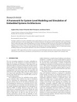
<span class='text_page_counter'>(14)</span><div class='page_container' data-page=14>

shared efficiently, and you do not need to purchase and install every device for every
computer. You can scan a picture from the scanner connected to the desktop in your
child's bedroom to the file server (a computer on the LAN with a high−capacity shared
hard disk) in your home office that also has the color printer attached it. Then you go
to the family room and use the imaging software on your notebook to edit and enhance
the picture while you recline in your favorite chair and watch TV surrounded by your
loved ones. After completing your first draft, you print the file on the printer attached
to the server in your office and review it. You then email the picture to your partner
through the Internet−sharing device and cable modem; you also leave a note for your
assistant with the file name. When your assistant comes in the next day, he or she
opens the file that you saved on the server from his or her workstation and makes the
final changes. Over the weekend your friends come over with their laptops and

802.11b Wi−Fi cards and you play network games over the wireless LAN.

<b>Figure 1.3: A SoHo wireless LAN setup [4]</b>
<i><b>1.3.2 Enterprise</b></i>

</div>
<span class='text_page_counter'>(15)</span><div class='page_container' data-page=15>

protected not only from outsiders but there is also the need to have proper access
control for authorized users. The speed and bandwidth requirements are also high, and
the network needs to be properly segmented to reduce the network traffic. An
enterprise network can also span across multiple floors, multiple buildings, and
multiple locations. There may be several Internet and VPN connection lines linking a
network with other parts of the enterprise network. There is also the need for covering
the complete office area without any dead zones (an area without a network signal) as
well as allowing the users to roam freely between floors, in the campus, and across
locations.

</div>
<span class='text_page_counter'>(16)</span><div class='page_container' data-page=16>

going into a meeting and then waiting for the presenter to connect their computers to
the projectors and fiddle with the projectors until they get started.[4]

<b>Figure 1.4: Enterprise wireless LAN setup</b>
<i><b>1.3.3 Wireless LAN Security Requirements</b></i>

</div>
<span class='text_page_counter'>(17)</span><div class='page_container' data-page=17>

within the one−mile radius can easily intercept the signal and possibly conduct an
attack on the network. A standalone wired LAN (one that is not connected to an
outside network) is far more secure when compared with a standalone wireless LAN.
Wireless LAN security can be compared to wired LAN security by using the example
of old cordless phones that did not securely communicate with their base stations. For
example, assume that your neighbor and you both have one of the old cordless phones
that did not encrypt the signals between the handset and the base station. Every time
you pick up the phone to make a phone call, provided that your and your neighbor's
phone were using the same frequency channel, you will be able to eavesdrop on your

neighbor's conversation. Wireless LANs are, therefore, inherently insecure and
appropriate measures must be taken to ensure a high−performance and secure wireless
LAN.

To secure a wireless LAN, both operational security (see Chapter 5, "Network
Security") and data security must be enforced. The security issues of wireless LANs
are similar to those of the wired LANs, and in this chapter, we discuss only the issues
that relate to operational security and the data security issues of the wireless LANs.
For more information on wired LAN security.

<i><b>1.3.4 Wireless LAN Operational Security Requirements</b></i>

Operational security of the wireless LANs deals with the security primitives
that provide a flawless operation of a wireless LAN. Operational security must be
implemented to avoid any threats that can affect the day−to−day operation of a
wireless LAN. Most such threats are possible due to poorly configured wireless LAN
setup, the inherent radio frequency−based transmission medium, the technologies and
the protocols used to transmit the data, or insufficient user authentication. In this
section, we look at the general security requirements that are necessary to ensure the
operational security of a wireless LAN. We also examine the need for securing
wireless access points (APs), the radio frequency (RF) methods that are used to
transmit data over the airwaves, link−level security that allows wireless equipment to
operate in a wireless LAN, and wireless LAN authentication. We also talk about the
most common known attacks on wireless LANs.

</div>
<span class='text_page_counter'>(18)</span><div class='page_container' data-page=18>

Most wireless LANs operate in infrastructure mode (see Chapter 2, "Wireless
LANs") where a wireless access point (AP) coordinates communication among its
users by acting as a hub and transmitting data received from one user to another. For
example, let's assume a wireless LAN that consists of two users (Alice and Bob) with
computers equipped with wireless LAN adapters (along with necessary software and

drivers) and an access point. In this example, when user Alice sends a message to user
Bob, Alice's wireless LAN adapter transmits the data to the AP, which in turn looks at
the data packet that is intended for Bob, and transmits the data to Bob. The use of APs
to route all the traffic among its users makes a wireless LAN less reliable, as all the
users on a given wireless LAN share the same AP. This may result in a single point of
failure, where anything happens to the AP. For example, if an AP gets too busy or it is
hacked, it affects the performance of the entire network. In addition to the
single−point−of−failure APs, most APs that are available today can be managed using
a wireless connection. This management feature, though extremely useful, allows an
adversary to attempt to break into the security of an AP and possibly take over its
operation.

The number and types of attacks on wireless APs has been growing steadily,
and will continue to do so as they become more popular and widespread in
deployment. These attacks are easy to launch and some can be difficult to detect on
your network via traditional means. The most commonly known attack on an AP is
conducted by a wireless LAN adapter that constantly sends messages to an AP, making
it so busy that it cannot reply to the messages sent by real users of a network. This
attack is known as a denial−of−service (DoS) or flood attack, as the AP is flooded with
bad requests from the rogue wireless LAN adapter making the AP too busy to service
genuine requests from authorized users. Besides flooding attacks, there are other
attacks—for example, AP administration attacks, in which an AP is highjacked by an
adversary who then controls all traffic through the AP. In scenarios where an AP
connects a wireless LAN to a wired LAN, more advanced attacks can be launched that
target the wireless LAN as well as the wired LAN to which the wireless LAN is
connected.

</div>
<span class='text_page_counter'>(19)</span><div class='page_container' data-page=19>

authentication mechanisms for authenticating both the network users and the users
who are allowed to manage the AP features. Carefully designed APs also contain
primitives for securing against DoS. More advanced APs come with a built−in router

and a firewall to prevent unauthorized traffic to enter the wireless LAN.

<i>Radio Frequency (RF) Method</i>

The data in a wireless LAN travels over the airwaves by using radio frequency
as the carrier. Using radio frequency as the carrier means the transmitting LAN device
—for example, a wireless LAN adapter—superimposes the data on a predefined radio
frequency and then transmits it over the air. The receiving LAN device separates the
data from the carrier wave, converts it into digital signal, and interprets accordingly.
The security of the data transmitted over the air can be affected in many ways, some of
which include: jamming the radio frequency, which makes a wireless LAN inoperable,
and eavesdropping on the authentication of the data, which reveals the user
information (the data security in a wireless LAN is discussed later in this chapter). A
typical wireless LAN has a range of up to 300 meters per AP. Under most
circumstances and depending on the placement of the AP, just like cordless phones, the
waves carrying the signals can easily penetrate through the walls. It is, therefore,
important that the APs be placed at or near the center of a wireless LAN site to reduce
the distance that the airwaves can travel.

The method used to transmit the data over the airwaves is also of prime
importance when considering the security of a wireless LAN. There are many different
methods used today to transmit the data in a wireless LAN. The most common are
direct−sequence spread spectrum (DSSS) and frequency−hopping spread spectrum
(FHSS). FHSS is considered more secure and resilient to attacks compared to DSSS.
In FHSS, the channel at which data is transmitted keeps switching, whereas in DSSS
the data is transmitted at a fixed channel. (For more information on radio frequency
methods, see Chapter 2.)

When choosing a wireless technology, it is important to choose a technology
that provides the best RF security primitives. The most current available wireless LAN

equipment—for example, 802.11−standard devices—utilizes the DSSS method.

</div>
<span class='text_page_counter'>(20)</span><div class='page_container' data-page=20>

Many wireless LANs authenticate users based on link−level authentication, in
which a network adapter in a wireless LAN communicates with an AP or with another
adapter that identifies itself using its media access control (MAC) address. MAC
addresses are 48 bits long, expressed as 12−hexadecimal digits (0 to 9, plus A to F,
capitalized). These 12−hex digits consist of the first 6 digits (which should match the
vendor of the Ethernet interface within the station) and the last 6 digits, which specify
the interface serial number for that interface vendor. These addresses are usually
written hyphenated by octets (for example, 12−34−56−78−9A−BC). By industry
standards, MAC addresses are burnt into and printed on the network adapters used to
communicate in a wireless. If configured properly, most wireless LAN APs are
designed so that they can authenticate a user based on the MAC identifiers that are
preprogrammed in the AP by the administrator. That means that APs let in only those
network adapters, and hence users, that identify themselves with known MAC
addresses. The MAC−based authentication is considered complex and cumbersome
because it requires every AP in a network to have the MAC address of every adapter
that might use the AP services. MAC−based authentication is also considered weak
because of the availability of LAN adapters that can be reprogrammed to use a
different MAC address. In such a case, a hacker acquires a wireless LAN adapter that
is programmable and reprograms the adapter to use a MAC address that is known by a
network he or she wants to attack. The hacker then conducts an attack by bringing his
or her computer equipped with a rouge LAN adapter within the radio range of the AP.
The LAN adapter with the forged MAC address leads the AP into believing that it is a
previously authorized network adapter and successfully gains access to the LAN.

MAC−based authentication should be used only as a supplementary
authentication method. If MAC−based authentication is used, the network becomes
vulnerable to such rogue wireless LAN adapters, which may impersonate an
authorized wireless LAN adapter to gain access to the network.

<i>Network Authentication</i>

</div>
<span class='text_page_counter'>(21)</span><div class='page_container' data-page=21>

LAN technologies do not include a robust mechanism for network authentication.
Most network technologies—for example, 802.11−standard devices—only allow a
service set identifier (SSID)−based authentication, in which each AP is assigned a
unique identifier consisting of letters and numbers and broadcasts this identifier to
show its presence. All wireless LAN devices use this identifier to communicate with
the AP.

The SSID−based authentication is extremely weak and only provides AP
identification. The SSIDs are easily programmable on most APs. An attack on APs,
known as rogue AP attack, is the most popular attack that involves an adversary
planting an AP in a wireless LAN with the SSID set to the one that is used by the
network users. If the network relies only on the SSID of an AP for its authentication,
the rogue AP successfully gains access to all the incoming traffic from wireless LAN
adapters that is addressed to the intended AP. More information on authentication
mechanisms used in 802.11 is provided in 802.11 WEP Authentication, later in this
chapter.

<i><b>1.3.5 Wireless LAN Data Security</b></i>

"Network Security," data in transit in an insecure medium must always be
protected using encryption primitives. Encryption−based data security is even more
important in wireless LAN, because without encryption the data is available for
examination to all authorized users and anyone who can receive the RF signals.

Most attacks on data security in a wireless LAN are conducted by analyzing the
LAN traffic. If the data is not transmitted in encrypted form, anyone can easily
eavesdrop upon, alter, or damage it. The data security of wireless LANs is further

degraded by the fact that most wireless LAN equipment today does not have security
features enabled by default. A user has to manually configure the security parameters,
which also inhibits the use of encryption in wireless LANs for data security.

</div>
<span class='text_page_counter'>(22)</span><div class='page_container' data-page=22>

<b>CHAPTER 2: SIGNAL PROPAGATION MODEL </b>
<b>IN WIRELESS LAN NETWORKS</b>

<b>2.1 IEEE 802.11 Standard family [6]</b>

12Equation Section 2First WLAN (Wireless Local Area Networks) experiment
using infrared links creating a local network in a factory was carried out by IBM in
1979, this technology was not ready; and the LAN explosion began mainly thanks to
the important emergence of the PC’s around 1983. In 1980 in order to create standards
to integrate different technologies and make them work together, the IEEE started
working in the 802 family standards (at the same time that the ISO carried out the OSI
model) predicting that this first explosion of the technology could last the next decades
as show in Figure 2.1. There is also important mention that the FCC deregulated the
band of 2.4-2.5 GHz giving chance to develop in this band in 1985. Wi-Fi is aimed at
use within unlicensed spectrum. This enables users to access the radio spectrum
without the need for the regulations and restrictions that might be applicable
elsewhere. The downside is that this spectrum is also shared by many other users and
as a result the system has to be resilient to interference.

<b>Figure 2.1: The relationship between the various components of the 802</b>
<b>family and their place in the OSI model</b>

</div>
<span class='text_page_counter'>(23)</span><div class='page_container' data-page=23>

IEEE 802.11 standard was born, aiming to provide a reliable, fast, inexpensive, robust
wireless solution that could grow into a standard with widespread acceptance, using
the regulated ISM band from 2.4-2.5 GHz; it wanted to appear identically to wired
LANs. With the invention of the 802.11n and the adoption of the MIMO technology,

in 2007 we have another big step forward in the used technology; the same as in the
2012 when thanks to the use of only the 5GHz band the data rates improve
dramatically and the use of the Wi-Fi connections focus on small cells with great
performances.

</div>
<span class='text_page_counter'>(24)</span><div class='page_container' data-page=24>

antenna receiving and the Channel Bonding technique permitting to combine two
non-overlapping channels of 20 MHz in one of 40 MHz for getting better data rates. The
802.11ac exploits more efficiently the features of the 802.11n: the OFDM technique,
uses a more dense modulation, amplifies the channel bonding technique for getting
bigger channel widths and also the MIMO is used with more antennas, and the variant
MU-MIMO is incorporated in the DL; obtaining in this case for the 5GHz band data
rates much more bigger. Finally we know so little about the 802.11ax, but by the
information about the data rates obtained; it exceeds by far the ones got by the
802.11ac.

<b> 2.2 RF signal propagation in Wireless LAN networks</b>
<i><b>2.2.1 Complex Modulation [6]</b></i>

Since digital radios are no longer dealing with analog information, they do not
have to be based on modulations that support analog signals. They merely have to
transit 1’s and 0’s. This can be done simply with two phase or amplitude states: one
state representing a binary 1, the other representing a 0. In order to transmit data faster,
you need more transitions. Luckily, because of the number of discrete phase angles
available (theoretically 360 but practically far less) and the number of amplitude states
available (theoretically infinite, but again practically far less), a carrier transition can
represent more than one bit. If four distinct carrier states are available, 2 bits can be
represented by each transition, eight states yield 3 bits, and so forth.

</div>
<span class='text_page_counter'>(25)</span><div class='page_container' data-page=25>

Quadrature Phase Shift Keying (QPSK) is the next logical step up the
modulation complexity curve. As shown in Figure below, QPSK uses four distinct

phases, each separated by 90 degrees. It can represent two bits per transition, but in
return requires more signal power at the receiver in order to recover the transmitted
information accurately. As previously discussed, there is no reason why one state must
be 0 degrees. As in BPSK, an initial state of 45 degrees is commonly used.

Further increases in efficiency can come from adding even more phase states.
Doubling the number of phase states in QPSK yields 8 PSK, which uses eight distinct
phases separated by 45 degrees, and can represent three bits per transition.

</div>
<span class='text_page_counter'>(26)</span><div class='page_container' data-page=26>

well. This is known as QAM, or Quadrature Amplitude Modulation and is a fancy
name for a simple process. If you take the two phase states of BPSK, and add two
distinct amplitude states to each, you have QAM. This concept is illustrated in Figure
below. The signal is a basic BPSK signal with 0 and 180 degree phase states, but now
each phase state is also transmitted with two unique amplitudes.

By adding two distinct amplitude shifts to a QPSK signal you get 8 QAM,
which has eight distinct phase/amplitude states. Each of these states can represent 3
bits per transition, the same as for 8 PSK. But wait, there’s still more! 16 QAM has
four phase states with four amplitude states, can represent 4 bits per transition, 32
QAM can represent 5 bits, 64 QAM can represent 6 bits, and 256 QAM, which has
sixteen phase states and sixteen unique amplitude states, can represent 8 bits per
transition. All of these modulations are commonly used in modern equipment. In fact
some modern point-to-point microwave equipment uses 512 QAM.

<i><b>2.2.2 OFDM</b></i>

</div>
<span class='text_page_counter'>(27)</span><div class='page_container' data-page=27>

spaced apart at precise frequencies so as to provide “orthogonality.” The center of the
modulated carrier is centered on the edge of the adjacent carriers. This technique
prevents the independent demodulators from seeing frequencies other than their own.
The benefits of OFDM are high spectral efficiency, great flexibility to conform to

available channel bandwidth, and lower susceptibility to multipath distortion. This is
useful because in a typical terrestrial

</div>
<span class='text_page_counter'>(28)</span><div class='page_container' data-page=28>

equipment. Just like all the other technologies we’ve discussed, the implementation
trade-offs are selected by the standards body or equipment designer in order to
maximize the equipment’s utility in a given market space. OFDM, because of its
flexibility and high spectral efficiency is being considered as the technology for 4th
generation cellular systems, and is being used in more and more standards-based and
proprietary data communications products. It is also the basis for wired ADSL
technology and some HDTV transmissions standards.

<i><b>2.2.3 Frequency Bands </b></i>

By law, the relation between the standard 802.11 and the frequency bands is
direct, without a deregulated frequency band there is no possibility to create a standard
working on these frequencies.

That is why in 1985, the FCC deregulated the spectrum from 2.4 GHz – 2.5
GHz for the ISM communities [7]. Almost fifteen years later the first version of 802.11
was working on that band, the same happened with the 5 GHz band some years later,
and actually the majority of the versions of the standard 802 are working on these two
bands.

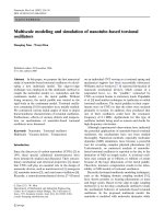
The 2.4 GHz band is divided in 11 or 13 channels of approximately 20 -22 MHz
(the ones available also depend on the laws of the country), but the useful ones are
those not affected by overlapping, ideally the 1, 7 and 13 for Europe or the 1,6 and 11
for USA.

<b>Figure 2.3: the 2.4GHz frequency band separated in the 14 channels</b>

</div>
<span class='text_page_counter'>(29)</span><div class='page_container' data-page=29>

At this point the MAC protocol CSMA/CA plays an important role; for standard
configuration of the 802.11 standard if there is a partial overlapping, the signal
overlapping is considered as noise for the transmitter of the original signal, while if
both signals are transmitted on the same channel the mechanism interprets that we
have two signals and the CDMA/CA is used; the main idea is that the transmitter
“listens” the channel before sending data for avoiding unnecessary collisions in the
long frames, this way there is a previous understanding between transmitter and
receiver for improving the communication but we also have higher delays.

If we can avoid the interference using different channels or thanks to the
CSMA/CA, why do we have to search for new frequency bands? The answer is easy,
despite of the different channels of the ISM band; the truth is that is a “free band” for
different uses and not only for the 802.11b/g/n standards. It causes interferences from
others devices using other protocols defined over the same band. Famous examples are
IEEE 802.15.1 (Bluetooth) or IEEE 802.15.4 (ZigBee), but not only those, also more
“simple” devices as car alarms, garage doors openers, microwave ovens, baby
monitors or digital cordless phones. Opinions of regulators and majors industry players
as Cisco, Google or Microsoft are clear[8]:

That is why the 5 GHz as an alternative has a lot of sense, a frequency band
almost free of interferences due to the few users in comparison of the crowded 2.4GHz
band that in addition permits higher bandwidth as shows Figure 4 using the channel
bonding technique. The use of this technique allows the user to dispose of a much
wider bandwidth, in conclusion more data rate available as Shannon proved in[9].

</div>
<span class='text_page_counter'>(30)</span><div class='page_container' data-page=30>

<b>Figure 2.4: Frequency and Performance</b>

Nowadays , the problem of the price since 802.11n is working also on 5 GHz
band is not as critical as it was, but recent studies as [8] showed how the increase of
the sales in devices using 5GHz band could saturate it (as the ISM band) in few years.

Also the predictions of the Wi-Fi Alliance showed that for 2015, 72 per cent of Wi-Fi
devices sold will operate in both 2.4 GHz and 5 GHz. That is why since April 2014
FCC is pressing for changing some laws (increase power (EIRP) on parts of 5GHz
band, or extend the 5.8 GHz band), also fighting against the auto industry lobby (due
to intelligent transportation systems live in 5.9 GHz)[11].

<b>2.3 RF signal propagation model [12]</b>
<i><b>2.3.1 Indoor Model:</b></i>

Because we use indoor environments, it has some problem is the signal
propagated from the transmitter antenna will experience many different signal
transformations and paths with a small portion reaching the receiver antenna.
Awareness of this process will assist the user to better understand radio performance
limitations. Much research and study is dedicated to the characterization of the signal
environment (Often referred to as channel characterization). A few propagation
fundamentals are reviewed in the following text.

<i><b>2.3.2 Mechanisms:</b></i>

</div>
<span class='text_page_counter'>(31)</span><div class='page_container' data-page=31>

wavelength) and sharp edges for a typical indoor scenario. As shown in equation
below, the free space wavelength at 2.4 GHz is 4.92 inches. This wavelength relative
to flat surfaces is sufficiently small for wave propagation mechanisms to hold true.
Typically, the distances between walls, floors and ceilings are on the order of 10 feet or
greater, and the office environment contains many vertical and horizontal edges and
surfaces.

+ Reflection: The propagated signal striking a surface will either be absorbed,
reflected, or be a combination of both. This reaction depends on the physical and
signal properties. Physical properties are the surfaces’ geometry, texture and material
composition. Signal properties are the arriving incident angle, orientation, and

wavelength. Perfect conductors will reflect all of the signal. Other materials will
reflect part of the incident energy and transmit the rest. The exact amount of
transmission and reflection is also dependent on the angle of incidence, material
thickness and dielectric properties. Major contributors to reflection are walls, floors,
ceilings and furniture.

+ Diffraction: A diffracted wave front is formed when the impinging transmitted
signal is obstructed by sharp edges within the path.

Diffraction occurs when obstacles are impenetrable by the radio waves. Based
on Huygen’s principle, secondary waves are formed behind the obstructing body even
though there is no line of site. Indoor environments contain many types of these edges
and openings, both orientated in the vertical and horizontal planes. Thus the resultant
diffracted signal is dependent on the geometry of the edge, the spatial orientation, as
well as dependent on the impinging signal properties. Such as amplitude, phase and
polarization. The result of diffraction of a wave at an obstacle edge is that the wave
front bends around and behind the obstacle edge. Diffraction is best demonstrated by
the radio signal being detected close to the inside walls around corners and hallways.
This phenomenon can also be attributed to the waveguide effect of signals propagating
down hallways.

</div>
<span class='text_page_counter'>(32)</span><div class='page_container' data-page=32>

construction contains pressed steel I-beams throughout the wall supports. Furthermore,
construction materials such as conduit for electrical and plumbing service can add to
the scattering effect.

<i><b>2.3.3 Path loss:</b></i>

Path loss is difficult to calculate for an indoor environment. Again, because of
the variety of physical barriers and materials within the indoor structure, the signal
does not predictably lose energy. The path between receiver and transmitter is usually

blocked by walls, ceilings and other obstacles. Depending on the building construction
and layout, the signal usually propagates along corridors and into other open areas. In
some cases, transmitted signals may have a direct path (Line-of-Site, LOS) to the
receiver. LOS examples of indoor spaces are; warehouses, factory floors, auditoriums,
and enclosed stadiums. In most cases the signal path is obstructed.

Related to penetration losses there is a coefficient (kw,in) which calculates the
number of penetrated walls. To achieve that value, it is important to have in mind that
the layout scenario generated is deterministic and known. So the code knows exactly
where the walls are located.

Number of penetrated walls (kw,in) is calculated by counting the walls crossing
this direct path. Lwi parameter remaining is related to the material of the walls and is
extracted from the standards:

Material Weights (mm) 2.4 Ghz 5Ghz

Concrete 102 18 dB 26 dB

Concrete 203 30 dB 55 dB

Brick 10 dB 15 dB

Thin glass 1-3 dB 0.7 dB

Thick glass 3-5 dB 0.1 dB

Wood 10 B

<b>Table 11</b>

<i><b>2.3.4 Free space loss:[12]</b></i>

</div>
<span class='text_page_counter'>(33)</span><div class='page_container' data-page=33>

<b>Figure 2.35: Free space model</b>
<i>FSPL</i> 4<i>d</i>








2

222\* MERGEFORMAT (.)
Where d is distance in meters between the transmitter and receiver, and
λ(lambda) is the wavelength in meters. This equation also implies that as the
frequency increases the loss will be proportionally higher. Relating frequency to

wavelength:
<i>c</i>
<i>f</i>
 

; where c is the speed of light, c = 3×108 m/s, and frequency, f =
cycles per second. For example, the wavelength of the 2.4 GHz sinusoid, λ=.125
meters, λ=12.5 centimeters or λ=4.92 inches.

Free space loss defined in decibels is :

<i>Freespaceloss=10xlog(FSPL)</i> _{323\* MERGEFORMAT (.)}
We can see that Free Space Loss (FSL) = 40 dB @ 1 meter and Free Space Loss
(FSL) = 60 dB @ 10 meter .

</div>
<span class='text_page_counter'>(34)</span><div class='page_container' data-page=34>

<b>Figure 2.5: Line of Site Path Loss</b>
<i><b>2.3.5 Line of Site Path Loss</b></i>

For a LOS office scenario, the path loss is given by

<i>PL FSLref n1*10*log(dtr)</i> _{424\* MERGEFORMAT (.)}
Where FSLref is the free space loss in dB determined in the far field of the
antenna. Usually for indoor environments, this is calculated to be 1 or 10 meters as
shown in equation (3). “dtr” is the distance between the receiver and transmitter. The
symbol “n1” is a scaling correction factor which is dependent on the attenuation of the
propagation environment. In this case, equation (4) is for large indoor spaces. The n1
factor has been determined from empirical data collected and can be found in the
excellent references by [13]. For line of site application in hallways the n1 factor has
been determined to be less than 2. This is due to the waveguide effect provided by
properties of hallways or corridors.

Figure 2.6 shows the free space attenuation in dB for a typical indoor
application. The curve represents various LOS path losses. The first segment
represents the path loss due to free space. The second and last segments represent a
more loss path. The instantaneous drop demonstrates the loss due to obstruction of the
LOS path.

<i><b>2.3.6 Obstructed Path Loss</b></i>

</div>
<span class='text_page_counter'>(35)</span><div class='page_container' data-page=35>

propagation phenomenon, the path loss models also account for the effects of different
building types. Examples are multi-level buildings with windows, or single level

buildings without windows.

<b>Figure 2.6: Path loss Between Building Floors</b>

It has been shown (See Figure 2.7) that the propagation loss between floors
begin to diminish with increasing separation of floors non-linearly. The attenuation
becomes less per floor as the number of floors increases. This phenomenon is thought
to be caused by diffraction of the radio waves alongside of a building as the radio
waves penetrate the building’s windows. Also, a variety of different indoor
configurations can be categorized for buildings with enclosed offices, or office spaces
consisting of a mix of cubicles and enclosed rooms. Examples of attenuation through
obstacles for various materials are shown in the table below.

</div>
<span class='text_page_counter'>(36)</span><div class='page_container' data-page=36>

<b>CHAPTER 3: MODELING AND SIMULATIONS</b>
<b>3.1 Simulation of signal propagation in WLAN</b>

<i><b>3.1.1 WLAN propagation overview</b></i>

53Equation Section 3 The main problem that exists for indoor environments is
that the signals propagated from the transmitter antenna will experiences many
different signal transformations and paths with a small portion reaching the receiver
antenna. Awareness of this process will assist the user to better understand radio
performance limitations. Much research and study is dedicated to the characterization
of the signal environment (Often referred to as channel characterization). A few
propagation fundamentals are reviewed in the following text.

<i><b>3.1.2 Simulations</b></i>
<i>Free Space Path Loss</i>

First, the free space path loss is computed as a function of propagation distance

and frequency. In free space, RF signals propagate at a constant speed of light in all
directions. At a far enough distance, the radiating source looks like a point in space
and the wavefront forms a sphere whose radius is equal to . The power density at the

wavefront is inversely proportional to <i>R</i>2
,

<i>P_t</i>
4<i>R</i>2

. <i>Where Pt</i> is the transmitted signal
power. For a monostatic radar where the signal has to travel both directions (from the
source to the target and back), the dependency is actually inversely proportional to <i>R</i>4,
as shown previously in the radar equation. The loss related to this propagation
mechanism is referred to as free space path loss, sometimes also called the spreading
loss. Quantitatively, free space path loss is also a function of frequency, given by [14]:

<i>L_fs</i> 20log(4<i>R</i>

 <i>)dB</i> _{636\* MERGEFORMAT (.)}
As a convention, propagation losses are often expressed in dB. This convention makes
it much easier to derive the two-way free space path loss by simply doubling the
one-way free space loss.

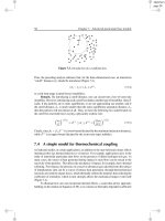
The following figure plots how the free space path loss changes over the frequency
between 10 to 1000 GHz for different ranges.

</div>
<span class='text_page_counter'>(37)</span><div class='page_container' data-page=37>

R0 = [100 1e3 10e3];
freq = (10:1000).'*1e9;
apathloss = fspl(R0,c./freq);

loglog(freq/1e9,apathloss);
grid on; ylim([90 200])

legend('Range: 100 m', 'Range: 1 km', 'Range: 10 km')
xlabel('Frequency (GHz)');

ylabel('Path Loss (dB)')
title('Free Space Path Loss')

<b>Figure 3.1: illustrates that the propagation loss increases with range and</b>
<b>frequency</b>

Propagation Loss Due to Rain

In reality, signals do not travel in a vacuum, so free space path loss describes
only part of the signal attenuation. Signals interact with particles in the air and lose
energy along the propagation path. The loss varies with different factors such as
pressure, temperature, water density.

</div>
<span class='text_page_counter'>(38)</span><div class='page_container' data-page=38>

The rain rate can range from less than 0.25 mm/h for very light rain to over 50 mm/h
for extreme rains. In addition, because of the raindrop’s shape and its relative size
compared to the RF signal wavelength, the propagation loss due to rain is also a
function of signal polarization.

The following plot shows how losses due to rain vary with frequency. The plot
assumes the polarization to be horizontal, so the tilt angle is 0. In addition, assume that
the signal propagates parallel to the ground, so the elevation angle is 0. In general,
horizontal polarization represents the worse case for propagation loss due to rain.
R0 = 1e3; % 1 km range

rainrate = [1 4 16 50]; % rain rate in mm/h

el = 0; % 0 degree elevation

tau = 0; % horizontal polarization

for m = 1:numel(rainrate)

rainloss(:,m) = rainpl(R0,freq,rainrate(m),el,tau)';
end

loglog(freq/1e9,rainloss); grid on;

legend('Light rain','Moderate rain','Heavy rain','Extreme rain', ...

'Location','SouthEast');
xlabel('Frequency (GHz)');

ylabel('Rain Attenuation (dB/km)')

</div>
<span class='text_page_counter'>(39)</span><div class='page_container' data-page=39>

<b>Figure 3.2: Rain Attenuation for Horizontal Polarization</b>

Similar to rainfall, snow can also have a significant impact on the propagation
of RF signals. However, there is no specific model to compute the propagation loss
due to snow. The common practice is to treat it as rainfall and compute the propagation
loss based on the rain model, even though this approach tends to overestimate the loss
a bit.

<i>Propagation Loss Due to Fog and Cloud</i>

Fog and cloud are formed with water droplets too, although much smaller
compared to rain drops. The size of fog droplets are generally less than 0.01 cm. Fog is
often characterized by the liquid water density. A medium fog with a visibility of
roughly 300 meters, has a liquid water density of 0.05 g/m^3. For heavy fog where the
visibility drops to 50 meters, the liquid water density is about 0.5 g/m^3. The
atmosphere temperature (in Celsius) is also present in the ITU model for propagation
loss due to fog and cloud[16].

The next plot shows how the propagation loss due to fog varies with frequency.
T = 15; % 15 degree Celsius

waterdensity = [0.05 0.5]; % liquid water density in g/m^3

</div>
<span class='text_page_counter'>(40)</span><div class='page_container' data-page=40>

fogloss(:,m) = fogpl(R0,freq,T,waterdensity(m))';
end

loglog(freq/1e9,fogloss); grid on;
legend('Medium fog','Heavy fog');
xlabel('Frequency (GHz)');

ylabel('Fog Attenuation (dB/km)')
title('Fog Attenuation');

<b>Figure 3.3: Fog Attenuation</b>
Note that in general fog is not present when it is raining.
<i>Propagation Loss Due to Atmospheric Gases</i>

Even when there is no fog or rain, the atmosphere is full of gases that still affect
the signal propagation. The ITU model[17] . describes atmospheric gas attenuation as
a function of both dry air pressure, like oxygen, measured in hPa, and water vapour

density, measured in g/m^3.

The plot below shows how the propagation loss due to atmospheric gases varies with
the frequency. Assume a dry air pressure of 1013 hPa at 15 degrees Celsius, and a
water vapour density of 7.5 g/m^3.

</div>
<span class='text_page_counter'>(41)</span><div class='page_container' data-page=41>

ROU = 7.5; % water vapour density in g/m^3

gasloss = gaspl(R0,freq,T,P,ROU);
loglog(freq/1e9,gasloss); grid on;
xlabel('Frequency (GHz)');

ylabel('Atmospheric Gas Attenuation (dB/km)')
title('Atmospheric Gas Attenuation');

<b>Figure 3.4: Atmospheric Gas Attenuation</b>

The plot suggests that there is a strong absorption due to atmospheric gases at
around 60 GHz. The next figure compares all weather related losses for a 77 GHz
automotive radar. The horizontal axis is the target distance from the radar. The
maximum distance of interest is about 200 meters.

R = (1:200).';
fc77 = 77e9;

apathloss = fspl(R,c/fc77);
rr = 16; % heavy rain

</div>
<span class='text_page_counter'>(42)</span><div class='page_container' data-page=42>

M = 0.5; % heavy fog

afogloss = fogpl(R,fc77,T,M);
agasloss = gaspl(R,fc77,T,P,ROU);

% Multiply by 2 for two-way loss

semilogy(R,2*[apathloss arainloss afogloss agasloss]);
grid on;

xlabel('Propagation Distance (m)');
ylabel('Path Loss (dB)');

legend('Free space','Rain','Fog','Gas','Location','Best')
title('Path Loss for 77 GHz Radar');

<b>Figure 3.5: Path loss for 77 GHz Radar</b>

The plot suggests that for a 77 GHz automotive radar, the free space path loss is
the dominant loss. Losses from fog and atmospheric gasses are negligible, accounting
for less than 0.5 dB. The loss from rain can get close to 3 dB at 180 m.

</div>
<span class='text_page_counter'>(43)</span><div class='page_container' data-page=43>

Functions mentioned above for computing propagation losses, are useful to establish
budget links. To simulate the propagation of arbitrary signals, we also need to apply
range-dependent time delays, gains and phase shifts.

The code below simulates an air surveillance radar operated at 24 GHz.
fc = 24e9;

First, define the transmitted signal. A rectangular waveform will be used in this case
waveform = phased.RectangularWaveform;

wav = waveform();

Assume the radar is at the origin and the target is at a 5 km range, of the direction of
45 degrees azimuth and 10 degrees elevation. In addition, assume the propagation is
along line of sight (LOS), a heavy rain rate of mm/h with no fog.

Rt = 5e3;
az = 45;
el = 10;

pos_tx = [0;0;0];

pos_rx = [Rt*cosd(el)*cosd(az);Rt*cosd(el)*sind(az);Rt*sind(el)];
vel_tx = [0;0;0];

vel_rx = [0;0;0];

loschannel = phased.LOSChannel(...

'PropagationSpeed',c,...

'OperatingFrequency',fc,...

'SpecifyAtmosphere',true,...

'Temperature',T,...

'DryAirPressure',P,...

'WaterVapourDensity',ROU,...

'LiquidWaterDensity',0,... % No fog
'RainRate',rr,...

'TwoWayPropagation', true)
loschannel =

</div>
<span class='text_page_counter'>(44)</span><div class='page_container' data-page=44>

PropagationSpeed: 299792458
OperatingFrequency: 2.4000e+10
SpecifyAtmosphere: true

Temperature: 15
DryAirPressure: 101300
WaterVapourDensity: 7.5000
LiquidWaterDensity: 0
RainRate: 16

TwoWayPropagation: true
SampleRate: 1000000
MaximumDistanceSource: 'Auto'

The received signal can then be simulated as
y = loschannel(wav,pos_tx,pos_rx,vel_tx,vel_rx);
The total loss can be computed as

L_total = pow2db(bandpower(wav))-pow2db(bandpower(y))
L_total =

289.6873

To verify the power loss obtained from the simulation, compare it with the
result from the analysis below and make sure they match.

Lfs = 2*fspl(Rt,c/fc);

Lr = 2*rainpl(Rt,fc,rr,el,tau);
Lg = 2*gaspl(Rt,fc,T,P,ROU);
L_analysis = Lfs+Lr+Lg
L_analysis = 289.6472
Multipath Propagation

Signals may not always propagate along the line of sight. Instead, some signals
can arrive at the destination via different paths through reflections and may add up
either constructively or destructively. This multipath effect can cause significant
fluctuations in the received signal.

</div>
<span class='text_page_counter'>(45)</span><div class='page_container' data-page=45>

unit, the signal not only propagates directly to the mobile unit but is also reflected
from the ground.

Assume an operating frequency of 1900 MHz, as used in LTE, such a channel
can be modeled as

fc = 1900e6;

tworaychannel = phased.TwoRayChannel('PropagationSpeed',c,...

'OperatingFrequency',fc);

Assume the mobile unit is 1.6 meters above the ground, the base station is 100
meters above the ground at a 500 meters distance. Simulate the signal received by the

mobile unit.

pos_base = [0;0;100];
pos_mobile = [500;0;1.6];
vel_base = [0;0;0];

vel_mobile = [0;0;0];

y2ray = tworaychannel(wav,pos_base,pos_mobile,vel_base,vel_mobile);
The signal loss suffered in this channel can be computed as

L_2ray = pow2db(bandpower(wav))-pow2db(bandpower(y2ray))
L_2ray = 109.1524

The free space path loss is given by

L_ref = fspl(norm(pos_mobile-pos_base),c/fc)
L_ref = 92.1673

The result suggests that in this configuration, the channel introduces an extra 17
dB loss to the received signal compared to the free space case. Now assume the mobile
user is a bit taller and holds the mobile unit at 1.8 meters above the ground. Repeating
the simulation above suggests that this time the ground reflection actually provides a 6
dB gain! Although free space path loss is essentially the same in the two scenarios, a
20 cm move caused a 23 dB fluctuation in signal power.

pos_mobile = [500;0;1.8];

y2ray = tworaychannel(wav,pos_base,pos_mobile,vel_base,vel_mobile);
L_2ray = pow2db(bandpower(wav))-pow2db(bandpower(y2ray))

</div>
<span class='text_page_counter'>(46)</span><div class='page_container' data-page=46>

L_ref = 92.1666

<i>Wideband Propagation in a Multipath Environment</i>

Increasing a system's bandwidth increases the capacity of its channel. This
enables higher data rates in communication systems and finer range resolutions for
radar systems. The increased bandwidth can also improve robustness to multipath
fading for both systems.

Typically, wideband systems operate with a bandwidth of greater than 5% of
their center frequency. In contrast, narrowband systems operate with a bandwidth of
1% or less of the system's center frequency.

The narrowband channel in the preceding section was shown to be very
sensitive to multipath fading. Slight changes in the mobile unit's height resulted in
considerable signal losses. The channel's fading characteristics can be plotted by
varying the mobile unit's height across a span of operational heights for this wireless
communication system. A span of heights from 10cm to 3m is chosen to cover a likely
range for mobile unit usage.

% Simulate the signal fading at mobile unit for heights from 10cm to 3m

hMobile = linspace(0.1,3);

pos_mobile = repmat([500;0;1.6],[1 numel(hMobile)]);
pos_mobile(3,:) = hMobile;

vel_mobile = repmat([0;0;0],[1 numel(hMobile)]);
release(tworaychannel);

y2ray = tworaychannel(repmat(wav,[1 numel(hMobile)]),...
pos_base,pos_mobile,vel_base,vel_mobile);

The signal loss observed at the mobile unit for the narrowband system can now be
plotted.

L2ray = pow2db(bandpower(wav))-pow2db(bandpower(y2ray));
plot(hMobile,L2ray);

xlabel('Mobile Unit''s Height (m)');
ylabel('Channel Loss (dB)');

</div>
<span class='text_page_counter'>(47)</span><div class='page_container' data-page=47>

grid on;

<b>Figure 3.6: Multipath Fading Observed at Mobile Unit(1)</b>

The sensitivity of the channel loss to the mobile unit's height for this
narrowband system is clear. Deep signal fades occur at heights that are likely to be
occupied by the system's users.

Increasing the channel's bandwidth can improve the communication link's
robustness to these multipath fades. To do this, a wideband waveform is defined with a
bandwidth of 10% of the link's center frequency.

bw = 0.10*fc;

pulse_width = 1/bw;
fs = 2*bw;

waveform = phased.RectangularWaveform('SampleRate',fs,...

'PulseWidth',pulse_width);
wav = waveform();

A wideband two-ray channel model is also required to simulate the multipath
reflections of this wideband signal off of the ground between the base station and the
mobile unit and to compute the corresponding channel loss.

</div>
<span class='text_page_counter'>(48)</span><div class='page_container' data-page=48>

phased.WidebandTwoRayChannel('PropagationSpeed',c,...

'OperatingFrequency',fc,'SampleRate',fs);

The received signal at the mobile unit for various operational heights can now
be simulated for this wideband system.

y2ray_wb = widebandTwoRayChannel(repmat(wav,[1 numel(hMobile)]),...
pos_base,pos_mobile,vel_base,vel_mobile);

L2ray_wb = pow2db(bandpower(wav))-pow2db(bandpower(y2ray_wb));
hold on;

plot(hMobile,L2ray_wb);
hold off;

legend('Narrowband','Wideband');

<b>Figure 3.7: Multipath Fading Observed at Mobile Unit (2)</b>

</div>
<span class='text_page_counter'>(49)</span><div class='page_container' data-page=49>

is increasing, reducing the amount of coherence between the two signals when

received at the mobile unit.

<i>Conclusion</i>

This example provides a brief overview of RF propagation losses due to
atmospheric and weather effects. It also introduces multipath signal fluctuations due to
bounces on the ground. It highlighted functions and objects to calculate attenuation
losses and simulate range-dependent time delays and Doppler shifts.

<b>3.2 Simulation of signal propagation in an area with multi-walls.</b>
<i><b>3.2.1 Indoor Propagation Models</b></i>

Ideally, for getting the optimal propagation model we should solve the Maxwell
equations (FDTD models) based on the information provided by the shape of the
objects present in the room/building. As this method would be highly complex
computationally, the deterministic models (based on Geometrical Optics) can be use as
an alternative. These models use the optical geometry and try to simulate the
environment, based on provided information of objects, focus direction and
illumination…

Although the results obtained by these deterministic models are used to be
satisfactory, the amount of data required which means a high time cost does not
compensate us.

That is the reason why the empirical models (COST, ITU…) are possible
alternatives. These models are based in measures previously done and try to generate a
pattern that can be useful to fully define the event. However, these models are not
complex enough to predict instantaneous changes or specific signal variations, for this
reason we would need the deterministic models. The positive part is that the
complexity required is much more reduced, and number of input parameters is small

compared with the previous model; that is why the computational cost is in
consequence also reduced.

</div>
<span class='text_page_counter'>(50)</span><div class='page_container' data-page=50>

the Motley-Keenan model were out of our purpose for their complexity and trade-off
precision-computational cost could not be as good as with the models provided here.
Even though there are more empirical models that could be useful apart of these as in
[18], we have focused on the “classical ones”.

The more interesting ones are the ITU-R P.1238-7 and the MWM, the rest are
too simple: the Free-Space Path Loss is the basic structure for modelling the wireless
system and the LAM or the 1SM just simply add one additional parameter for
modelling the others losses, which is not enough complex for obtaining accurate
results. The others, as mentioned, are outside our study.

Some studies show a similar performance between the ITU-R P.1238-7 and the
COST231 MWC for different scenarios, that is why for simplicity and computational
time we have chosen a modified version of the ITU model, due to we are interested in
flat layout models representing only one floor (considering only the losses due to walls
and not to floors). That is why we will focus on these two models in this Project.

The ITU-R P.1238 [12] models the Loss using as a parameters the frequency (),
the distance ( ), the distance power loss coefficient ( ) and the penetration Loss factor
() which depends on the frequency and the number of floors between the transmitter
and receiver ( ). There is important to mention that these parameters have been
empirically found and also say that must be greater than 1 meter for the validity of
this model as we can see again in[12]:

<i>L(dB) 20log( f ) Nlog(d) L_f(n)</i>28 _737\*
MERGEFORMAT (.)

Values used for this model are:

For our work bands (2.4 GHz and 5 GHz) we have this parameters based on various
measurement results found in[12]:

Power Loss Coefficient N:

<b>Frequency (GHz) </b> <b>Residential </b> <b>Office </b>

2.4 28 30

5 28-30* 31

*: depending on the materials used in the walls (concrete or wooden)

Floor penetration loss factors, <i>L nf</i>( )(dB) with n being the number of floors penetrated,

</div>
<span class='text_page_counter'>(51)</span><div class='page_container' data-page=51>

<b>Frequency (GHz) </b> <b>Residential </b> <b>Office </b>

2.4 5-10* 14

5 713* 16

Table: Floor Penetration Loss Factor for different environments and frequencies

*: depending on the materials used in the walls (5 or 7 for each wooden Wall, 10 or 13
for each concrete wall)

The COST-231 Multi-Wall Model (MWM)[12], as it is showed in Equation 2
and Equation 3 gives the path loss as the free space loss (<i>L n dfs</i>( , )) added with losses

introduced by the walls and floors penetrated by the direct path between the
transmitter and the receiver. This model considers different types of walls ( <i>Kwi</i> )
depending on their losses ( <i>Lwi</i> , penetration losses) but always the same type of floors

(
2
( )
1
<i>f</i>
<i>f</i>
<i>K</i>
<i>b</i>
<i>K</i>
<i>f</i> <i>f</i>
<i>K</i> <i>L</i>




). It has been observed that the total floor loss is a non-linear function of
the number of penetrated floors. This is compensated by adding an empirical
parameter b (usually around 0.5). Also we have n as a power decay index and as a
Loss constant. The multiwall model (MWM) can then be expressed in form:

<i>L(dB) L_fs</i>(n,d)<i> L_c</i> <i>L_wi</i>
<i>i</i>1

<i>N</i>



<i>K_wi K_f</i>(
<i>K_f</i>2
<i>K_f</i>1<i>b)</i>

<i>L_fa</i>

838\*
MERGEFORMAT (.)

<i>L_fs</i>(n,d) 10* n*log₁₀(4

 ) _{939\* MERGEFORMAT (.)}
<i><b>3.2.2 Simulation</b></i>

</div>
<span class='text_page_counter'>(52)</span><div class='page_container' data-page=52>

<b>Figure 3.8: One AP in an area with multiwall</b>

As seen on the picture, the signal level of wifi coverage. Placed in the corner
between the two walls with high wave breaking help the wifi can pass the next room.
The corner of the rest is made of materials with less break wave so the wifi is less
attenuated and can still be covered. Although, could not pass the next wall.

</div>
<span class='text_page_counter'>(53)</span><div class='page_container' data-page=53>

<b>Figure 3.10: Three AP set in different places.</b>

</div>
<span class='text_page_counter'>(54)</span><div class='page_container' data-page=54>

<b>Figure 3.12: Four AP set in different places.</b>

By changing AP pointers on Matlab simulation software, from there we have to
figure out how to optimize the wifi system.

<b>….</b>

<b>Conclusion and Recommendation</b>

<b>3. Experience and benefits learned from the study of topic:</b>
 Proficiency in C programming language, Matlab

 Understand the latest wireless networking technologies and how to operate a
wifi system.

 Proficient in simulation methods, modeling a signal system.
<b>4. Conclusion: </b>

</div>
<span class='text_page_counter'>(55)</span><div class='page_container' data-page=55>

how attraction and retention interventions work, using a systems perspective. It starts
with a common set of indicators, which enable comparison between various cases, and
facilitates reviews of real situations.

<b>References</b>

[1] a. A. I. M. Scott R. Fluhrer, "" Weaknesses in the key scheduling algorithm of
rc4. In SAC ’01: Revised Papers from the 8th Annual International Workshop
on Selected Areas in Cryptography,"" 2001.

[2] S. Sotillo, "Handbook of Computer Communications Standards, 2nd edition,
volume 2," 1990.

[3] C.-Y. H. Alan Holt, "802.11 Wireless Networks: Security and Analysis
Computer Communications and Networks," (in English), p. 212, 2010.

[4] A. K. Jahanzeb Khan, "Building Secure Wireless Networks with 802.11," (in
English), 2003.

[5] S. Fluhrer, I. Mantin, and A. Shamir, "Weaknesses in the Key Scheduling
Algorithm of RC4, Eighth Annual Workshop on Selected Areas in
Cryptography," 2001.

[6] Ron_Olexa, ""Implementing_802.11,_802.16_and_802."."

[7] <i>J. Berg, The IEEE 802.11 Standardization – Its History, Specifications,</i>
<i>Implementations, and Future (Technical Report GMU-TCOM-TR-8, George</i>
Mason University).

[8] "Globalstar Value Proposition," Globalstar Spectrum Holdings - Investor
Relations Solutions," 2014.

[9] Wikipedia, "Shannon–Hartley theorem, Available at:
2015.
[10] J. Berg, "The IEEE 802.11 Standardization – Its History, Specifications,

Implementations, and Future (Technical Report GMU-TCOM-TR-8, George
Mason University)."

[11] C. Gabriel, ""Towards 2020: Emerging Opportunities for Wi-Fi Services,"
Maravedis-Rethink," 2015.

[12] S. J. Park, C. H. Lee, K. T. Jeong, H. J. Park, J. G. Ahn, and K. H. Song,
"Fiber-to-the-home services based on wavelength-division-multiplexing passive
<i>optical network," IEEE Journal of Lightwave Technology, vol. 22, pp. </i>
2582-2591, 2004.

[13] T. S. Rappaport, ""Wireless Communications Principles and Practice," IEEE
Press/Prentice Hall PTR, Upper Saddle River, New Jersey," 1996.

[14] "Recommendation ITU-R P.525-2," 1994.

</div>
<span class='text_page_counter'>(56)</span><div class='page_container' data-page=56>

[16] "Recommendation ITU-R P.840-3," 2013.
[17] "Recommendation ITU-R P.676-10," 2013.

[18] R. E. e. al, ""A new generic model for signal propagation in Wi-Fi and Wimax
environments", in Wireless Days," 2008

</div>

<!--links-->