- Trang chủ >>
- Mầm non >>
- Mẫu giáo lớn
Chapter 2: Transmission Lines
Bạn đang xem bản rút gọn của tài liệu. Xem và tải ngay bản đầy đủ của tài liệu tại đây (1.8 MB, 52 trang )
<span class='text_page_counter'>(1)</span><div class='page_container' data-page=1>
<b>Bài giảng:</b>
<b>TRƯỜNG ĐIỆN TỪ (CT361)</b>
<b> (ELECTROMAGNETICS)</b>
<b>Chapter 2: </b>
<b>Transmission Lines</b>
<b> (Đường dây truyền sóng)</b>
<b>Giảng viên: GVC.TS. Lương Vinh Quốc Danh</b>
Bộ môn Điện tử Viễn thông, Khoa Cơng Nghệ
</div>
<span class='text_page_counter'>(2)</span><div class='page_container' data-page=2>
•
<i>Lumped-Element (phần tử tập trung) Model of </i>
Transmission Lines
•
Transmission-Line Equations
•
Wave Propagation on a Transmission Line
•
<i>Input Impedance (trở kháng ngõ vào) of the Lossless Line </i>
•
Special Cases of Lossless Line
•
Power Flow on a Lossless Transmission Line
•
<i>Transients (Quá độ) on Transmission Lines</i>
</div>
<span class='text_page_counter'>(3)</span><div class='page_container' data-page=3></div>
<span class='text_page_counter'>(4)</span><div class='page_container' data-page=4>
Transmission line parameters, equations
Vg(t) VAA’(t) VBB’(t)
A
A’ <sub>B’</sub>
B
<b>L</b>
VBB’(t) = VAA’(t-td) = VAA’(t-L/c)
= V<sub>0</sub>cos((t-L/c))
= V<sub>0</sub>cos(t- 2L/),
<i>Recall: =c/f, and = 2 </i>
<b>If >> L, V</b>BB’(t) V<sub>0</sub>cos(t) = VAA’(t),
<b>If <= L, V</b>BB’(t) VAA’(t) The circuit theory has to be replaced.
</div>
<span class='text_page_counter'>(5)</span><div class='page_container' data-page=5>
<b>Propagation Modes</b>
<b>Electric</b> and <b>magnetic</b> fields
<i>oscillate together but perpendicular </i>
to each other and the
electromagnetic wave moves in a
<i>direction perpendicular to both of </i>
<i><b>the fields. TEM modes </b></i>
</div>
<span class='text_page_counter'>(6)</span><div class='page_container' data-page=6>
<b>TEM transmission lines</b>
<b>Propagation Modes (cont.)</b>
d) Strip line e) Microstrip line
Metal
Dielectric spacing Metal ground
</div>
<span class='text_page_counter'>(7)</span><div class='page_container' data-page=7>
<b>Lumped-Element Model</b>
• Represent transmission lines as parallel-wire configuration
Vg(t) <sub>V</sub><sub>AA’</sub><sub>(t)</sub> <sub>V</sub>BB’(t)
A
A’ B’
B
z z z
</div>
<span class='text_page_counter'>(8)</span><div class='page_container' data-page=8>
<b>Transmission line equations</b>
• Represent transmission lines as parallel-wire configuration
V(z,t) = R’z <i>i</i>(z,t) + L’z <i>i</i>(z,t)/ t + V(z+ z,t), (2.12)
V(z,t)
<b>R’z</b> <b>L’z</b>
<b>G’z</b> <b><sub>C’z</sub></b> V(z+ z,t)
<i>i</i>(z,t) <i>i</i>(z+z,t)
<i>i</i>(z,t) = G’z V(z+ z,t) + C’z V(z+ z,t)/t + <i>i</i>(z+z,t), (2.15)
<b>FOUR transmission line parameters: Resistance R’ (Ω/m); Inductance L’ (H/m); </b>
Capacitance C’ (F/m); Conductance G’ (S/m)
</div>
<span class='text_page_counter'>(9)</span><div class='page_container' data-page=9>
• Transmission line equations
V(z,t) = R’z <i>i</i>(z,t) + L’z <i>i</i>(z,t)/ t + V(z+ z,t), (2.12)
V(z,t)
R’z L’z
G’z <sub>C’z</sub> V(z+ z,t)
<i>i</i>(z,t) <i>i</i>(z+z,t)
-V(z+ z,t) + V(z,t) = R’z <i>i</i>(z,t) + L’z <i>i</i>(z,t)/ t
- V(z,t)/z = R’ <i>i</i>(z,t) + L’ <i>i</i>(z,t)/ t, (2.14)
<i>Rewrite V(z,t) and i</i>(z,t)<i> as phasors, for sinusoidal V(z,t) and i</i>(z,t):
V(z,t) = Re( V(z) ejt), <i>i (z,t) = Re( i (z) e</i>jt),
</div>
<span class='text_page_counter'>(10)</span><div class='page_container' data-page=10>
• Transmission line equations
V(z,t)
R’z L’z
G’z <sub>C’z</sub> V(z+ z,t)
<i>i</i>(z,t) <i>i</i>(z+z,t)
Recall:
<i>di(t)/dt</i> = <i><sub>Re(d i e jt )/dt</sub></i> <i>= Re(i</i> je jt ),
- V(z,t)/z = R’ <i>i</i>(z,t) + L’ <i>i</i>(z,t)/ t, (2.14)
- dV(z)/dz = R’ <i>i</i>(z) + jL’ <i>i</i>(z), (2.18a)
</div>
<span class='text_page_counter'>(11)</span><div class='page_container' data-page=11>
• Transmission line equations
V(z,t)
R’z L’z
G’z <sub>C’z</sub> V(z+ z,t)
<i>i</i>(z,t) <i>i</i>(z+z,t)
<i>- i (z+ </i>z,t) + <i>i (z,t)</i> = G’z V(z + z ,t) + C’z V(z + z,t)/ t
- <i>i(z,t)/</i>z = G’ V(z,t) + C’ V(z,t)/ t, (2.16)
<i>Rewrite V(z,t) and i</i>(z,t)<i> as phasors, for sinusoidal V(z,t) and i</i>(z,t):
V(z,t) = Re( V(z) ejt), <i>i (z,t) = Re( i (z) e</i>jt),
<i>i</i>(z,t) = G’z V(z+ z,t) + C’z V(z+ z,t)/t + <i>i</i>(z+z,t), (2.15)
</div>
<span class='text_page_counter'>(12)</span><div class='page_container' data-page=12>
• Transmission line equations
V(z,t)
R’z L’z
G’z <sub>C’z</sub> V(z+ z,t)
<i>i</i>(z,t) <i>i</i>(z+z,t)
Recall:
dV(t)/dt = Re(d V e jt )/dt = Re(Vje jt ),
- <i>i(z,t)/</i>z = G’ V(z,t) + C’ V(z,t)/ t,
- d <i>i(z)/</i>dz = G’ V(z) + jC’ V(z), (2.18b)
</div>
<span class='text_page_counter'>(13)</span><div class='page_container' data-page=13>
<b>Telegrapher’s equation</b>
V(z,t)
R’z L’z
G’z C’z V(z+ z,t)
<i>i</i>(z,t) <i>i</i>(z+z,t)
- d <i>i(z)/</i>dz = G’ V(z) + jC’ V(z), (2.18b)
- dV(z)/dz = R’ <i>i</i>(z) + jL’ <i>i</i>(z), (2.18a)
• Telegrapher’s equation in phasor domain
Take d /dz on both sides of eq. (2.18a)
</div>
<span class='text_page_counter'>(14)</span><div class='page_container' data-page=14>
- d <i>i(z)/</i>dz = G’ V(z) + jC’ V(z), (2.18b)
- dV(z)/dz = R’ <i>i</i>(z) + jL’ <i>i</i>(z), (2.18a)
• Telegrapher’s equation in phasor domain
substitute (2.18b) to (2.19)
d²V(z)/dz² = (R’ + jL’) (G’+ jC’)V(z),
- d²V(z)/dz² = R’ d<i>i</i>(z)/dz + jL’ d<i>i</i>(z)/dz, (2.19)
d²V(z)/dz² - (R’ + jL’) (G’+ jC’)V(z) = 0, (2.20)
or
d²V(z)/dz² - ²V(z) = 0, (2.21)
² = (R’ + jL’) (G’+ jC’),
</div>
<span class='text_page_counter'>(15)</span><div class='page_container' data-page=15>
V(z,t)
R’z L’z
G’z C’z V(z+ z,t)
<i>i</i>(z,t) <i>i</i>(z+z,t)
- d <i>i(z)/</i>dz = G’ V(z) + jC’ V(z), (2.18b)
- dV(z)/dz = R’ <i>i</i>(z) + jL’ <i>i</i>(z), (2.18a)
• Telegrapher’s equation in phasor domain
Take d /dz on both sides of eq. (2.18b)
- d² <i>i(z)/</i>dz² = G’ dV(z)/dz + jC’ dV(z)/dz, (*)
</div>
<span class='text_page_counter'>(16)</span><div class='page_container' data-page=16>
substitute (2.18a) to (*)
d² <i>i(z)/</i>dz² = (R’ + jL’) (G’+ j<i>C’)i(z), </i>
d² <i>i(z)/</i>dz² - (R’ + jL’) (G’+ j<i>C’) i(z) = 0, </i>
or
d² <i>i(z)/</i>dz² - ²<i>i(z) = 0, </i> (2.23)
² = (R’ + jL’) (G’+ jC’),
- d² <i>i(z)/</i>dz² = G’ dV(z)/dz + jC’ dV(z)/dz, (*)
- d <i>i(z)/</i>dz = G’ V(z) + jC’ V(z), (2.18b)
- dV(z)/dz = R’ <i>i</i>(z) + jL’ <i>i</i>(z), (2.18a)
• Telegrapher’s equation in phasor domain
</div>
<span class='text_page_counter'>(17)</span><div class='page_container' data-page=17>
• Wave equations
d² <i>i(z)/</i>dz² - ²<i>i(z) = 0, </i> (2.23)
d²V(z)/dz² - ²V(z) = 0, (2.21)
<b> = + j, </b>Complex propagation constant
= Re (R’ + jL’) (G’+
jC’) ,
= Im (R’ + jL’) (G’+
jC’) ,
<b>Wave Equations</b>
</div>
<span class='text_page_counter'>(18)</span><div class='page_container' data-page=18>
<b>Telegrapher’s equation (cont.)</b>
V(z) = V0 (2.26a)
Solving the second order differential equation (2.21), (2.23):
+
<i><sub>e</sub></i>
-z+
V-0<i>e</i>
z<i>i(z) = </i>I+0
<i>e</i>
-z+
I<sub>0</sub>-<i>e</i>
z (2.26b)where:
+
V0 and V-0 are determined by boundary conditions.
+
</div>
<span class='text_page_counter'>(19)</span><div class='page_container' data-page=19>
• Characteristic impedance Z0
I0+ =
(R’ + jL’)
V+0
I0- =
(R’ + jL’)
-
V-0
= (R’ + jL’)
+
<b>Z0 </b>
Define characteristic impedance Z0
I0+
V0
=
= (R’ + jL’) (G’+ jC’)
(R’ + jL’)
(G’+j C’)
recall:
<b>Characteristic impedance Z</b>
<b><sub>0</sub></b></div>
<span class='text_page_counter'>(20)</span><div class='page_container' data-page=20>
• Example 2-1, an air line :
Solution:
R’ = G’ = 0, Z0<i> = 50 , = 20 rad/m, f = 700 MHz </i>
L’ = ? and C’ = ?
Z0 = <sub>(G’+j C’)</sub>(R’ + jL’) =
L’
C’ = 50
= (R’ + jL’) (G’+ jC’) = j <sub>L’C’</sub>
= + j,
= L’C’ = 20 rad/m
</div>
<span class='text_page_counter'>(21)</span><div class='page_container' data-page=21>
• Lossless transmission line :
= (R’ + jL’) (G’+ jC’)
= + j,
If R’<< j L’ and G’ << jC’,
<b>Lossless Transmission Lines </b>
Then:
(2.35)
</div>
<span class='text_page_counter'>(22)</span><div class='page_container' data-page=22>
<b>Phase velocity</b>
<b>Wavelength</b>
<b>Lossless Transmission Lines (cont.)</b>
(2.39)
(2.40)
</div>
<span class='text_page_counter'>(23)</span><div class='page_container' data-page=23>
<b>Reflection Coefficient </b>
<i>i(z) = </i>
V(z) = V+0
+
V0-<i>e</i>
jz<i>-e</i>
-jz<i>e</i>
-jz+
V0
Z0
<i>e</i>
jz
-V0
Z0
VL = = <sub>V</sub>+<sub>0</sub>
<sub>+</sub>
<sub>V</sub>-<sub>0</sub>V(z)
z = 0
-+
V0
Z0
-V0
Z0
<i>i(z)</i>
z = 0
<i>i</i>L = =
ZL = VL
<i>i</i>L
=
+
-V0
+
V0
-+
V0
Z
-V0
Z
+
V0
-V0 =
ZL - Z0
ZL + Z0
</div>
<span class='text_page_counter'>(24)</span><div class='page_container' data-page=24>
• Voltage reflection coefficient :
• Current reflection coefficient :
</div>
<span class='text_page_counter'>(25)</span><div class='page_container' data-page=25>
• <b>Example 2-2 :</b>
A’
z = 0
A
Z0 = 100
RL = 50
CL = 10pF
<i>f = 100 MHz</i>
ZL = RL + j/CL = 50 – j159 (Ohms)
</div>
<span class='text_page_counter'>(26)</span><div class='page_container' data-page=26>
<b>Standing Waves </b>
• From (2.44), we have:
|V(z)| = |V+0| |
<i>e</i>
-jz+
||<i>e</i>
jr<i>e</i>
jz|= |V+0| [1+ | |² + 2||cos(2z + r)]
1/2
-V0
+
V0
with =
(2.52)
|V(z)| is a function of <b> ~</b> <i>z</i>.
<i>• A similar expression can be derived for |I(z)| </i>
<b> ~</b>|I(z)| = |V+0|/|Z0| [1+ | |² - 2||cos(2z + r)]
1/2
</div>
<span class='text_page_counter'>(27)</span><div class='page_container' data-page=27>
<b>Standing Waves (cont.) </b>
The repetition period
of the standing wave
pattern is /2.
When voltage is a
<i>maximum</i>
, current is a
</div>
<span class='text_page_counter'>(28)</span><div class='page_container' data-page=28>
•
<b>Special cases</b>
1. ZL= Z0, = 0
= |V+0|
|V(z)|
</div>
<span class='text_page_counter'>(29)</span><div class='page_container' data-page=29>
2. ZL= 0, <b>short circuit</b>, = -1
= |V+0| [2 + 2cos(2z + )]
1/2
|V(z)|
<b>Standing Waves (cont.) </b>
3. ZL= ,<b>open circuit</b>, = 1
= |V+0| [2 + 2cos(2z )]
1/2
</div>
<span class='text_page_counter'>(30)</span><div class='page_container' data-page=30>
•
<b>Voltage maximum</b>
= |V+0| [1+ | |² + 2||cos(2z + r)] 1/2
|V(z)|
|V0+| [1+ | |],
|V(z)|<sub>max</sub> <sub>=</sub>
when 2z + r = - 2n.
<b>Standing Waves (cont.) </b>
</div>
<span class='text_page_counter'>(31)</span><div class='page_container' data-page=31>
•
<b>Voltage minimum</b>
<b>Standing Waves (cont.) </b>
</div>
<span class='text_page_counter'>(32)</span><div class='page_container' data-page=32>
<b>Voltage standing-wave ratio VSWR </b>
1 - | |
|V(z)|<sub>min</sub>
<b>S</b> |V(z)|max
=
1 + | |S = 1, when = 0,
S = , when || = 1,
(2.59)
<i><b>Example 2-4: 50-Ohm transmission line, Z</b></i><sub>L</sub><i> = 100 + j50 (Ω). Find , SWR.</i>
</div>
<span class='text_page_counter'>(33)</span><div class='page_container' data-page=33>
<b>Input Impedance of the Lossless Line</b>
Vg(t) <sub>V</sub><sub>L</sub>
A
z = 0
B
<i>l</i>
ZL
<i>z = - l</i>
Z0
Vi
Zg Ii
Zin(z) = Vi(z)
I<sub>i</sub>(z)
=
+
+
<i>e</i>
jz<i>e</i>
-jzV0( )
+
-
<i>e</i>
jz<i>e</i>
-jzV0( )
Z0 =
+
(1
<i>e</i>
j2z )-(1
<i>e</i>
j2z ) Z0+
(1
<i>e</i>
-j2 )<i>l</i></div>
<span class='text_page_counter'>(34)</span><div class='page_container' data-page=34>
A 1.05-GHz generator circuit with series impedance Zg = 10- and voltage source
given by Vg(t) = 10 sin(t +30º) is connected to a load Z<sub>L</sub> = 100 +j5 () through
a 50-, 67-cm long lossless transmission line. The phase velocity is 0.7c. Find
<i>V(z,t) and i(z,t) on the line. </i>
Solution:
<i>Since, Vp = ƒ, = Vp/f = 0.7c/(1.05 x 10</i>9<sub>) = 0.2 m. </sub>
= 2/, = 10 .
= (ZL-Z0)/(ZL+Z0), = 0.45exp(j26.6º)
+
(1
<i>e</i>
-j2 )<i>l</i>-(1
<i>e</i>
-j2 )<i>l</i> Z0Zin<i>(-l) =</i> = 21.9 + j17.4
V+0[exp(-j<i>l)+ </i>exp(j<i>l)</i>] <sub>=</sub>
Zin<i>(-l) + Zg</i>
Zin<i>(-l)</i>
Vg
</div>
<span class='text_page_counter'>(35)</span><div class='page_container' data-page=35>
<b>Short-circuited Line</b>
ZL= 0, = -1, S =
Vg(t) <sub>V</sub><sub>L</sub>
A
z = 0
B
<i>l</i>
ZL = 0
<i>z = - l</i>
Z0
Zg Ii
<b>Zin</b>
<b>sc</b>
<i>I(z) = </i>
V(z) = V0
<i>- e</i>
)jz+
(
<i>e</i>
-jz(
<i>e</i>
-jz+
V0
Z0
<i>e</i>
jz <sub>)</sub>
= -2jV+0sin(z)
= 2V+0cos(z)/Z0
Zin = <i>V(-l)</i>
<i>I(-l)</i> <i>= jZ</i>0.<i>tan(l)</i>
sc
(2.67)
</div>
<span class='text_page_counter'>(36)</span><div class='page_container' data-page=36>
<b>Short-circuited Line (cont.)</b>
Zin = <i>V(-l)</i>
</div>
<span class='text_page_counter'>(37)</span><div class='page_container' data-page=37>
Zin = <i>V(-l)</i>
<i>i(-l)</i> = jZ0<i>tan(l)</i>
<i>• If tan(l) >= 0, the line appears inductive, jL</i>eq = jZ0<i>tan(l), </i>
<i>• If tan(l) <= 0, the line appears capacitive, 1/(jC</i>eq)= jZ0<i>tan(l), </i>
<i>l = 1/[- tan (1/C</i>-1 eqZ0)],
• The minimum length results in transmission line as a capacitor:
<b>Short-circuited Line (cont.)</b>
L
</div>
<span class='text_page_counter'>(38)</span><div class='page_container' data-page=38>
<i>tan (l) = - 1/C</i>eqZ0 = -0.354,
Choose the length of a shorted 50- lossless line such that its input impedance
at 2.25 GHz is equivalent to the reactance of a capacitor with capacitance
C<sub>eq </sub>= 4pF. The wave phase velocity on the line is 0.75c.
Solution:
<i>Vp = ƒ, = 2/ = 2ƒ/Vp = 62.8 (rad/m) </i>
<i>l = 2l / = tan (-0.354) + n = - 0.34 + n </i>-1
</div>
<span class='text_page_counter'>(39)</span><div class='page_container' data-page=39>
ZL = 0, = 1, S =
z = 0
<i>z = - l</i>
Vg(t) <sub>V</sub><sub>L</sub>
A B
<i>l</i>
ZL =
Z0
Z<sub>g</sub> Ii
Zin
oc
<i>I(z) = </i>
V(z) = V0
<i>+ e</i>
)jz-(
<i>e</i>
-jz(
<i>e</i>
-jz+
V0
Z0
<i>e</i>
jz <sub>)</sub>
= 2V+0cos(z)
= 2jV+0sin(z)/Z0
Zin = <i>V(-l)</i>
<i>I(-l)</i> <i>= -jZ</i>0.<i>cot(l)</i>
oc
<b>Open-circuited Line (cont.)</b>
(2.72)
</div>
<span class='text_page_counter'>(40)</span><div class='page_container' data-page=40>
<b>Open-circuited Line (cont.)</b>
Zin = <i>V(-l)</i>
<i>I(-l)</i> <i>= -jZ</i>0.<i>cot(l)</i>
</div>
<span class='text_page_counter'>(41)</span><div class='page_container' data-page=41>
<b>Line of Length n/2</b>
= ZL
<i>tan(l) = tan[(2/)(</i>n/2)] = 0,
+
(1
<i>e</i>
-j2 )<i>l</i>-(1
<i>e</i>
-j2 )<i>l</i> Z0Zin<i>(-l) =</i>
Any multiple of half-wavelength line <b>doesn’t modify </b>the load impedance.
Vg(t)
A
z = 0
B
<i>l = n</i><i>/2</i>
<b>ZL</b>
<i>z = - l</i>
Z0
<b>Zin</b>
</div>
<span class='text_page_counter'>(42)</span><div class='page_container' data-page=42>
<i>Quarter-wave transformer: l = /4 + n/2</i>
<i>l = (2/)(/4 + n/2) = /2 , </i>
<b>= Z0²/ZL</b>
+
(1
<i>e</i>
-j2 )<i>l</i>-(1
<i>e</i>
-j2 )<i>l</i> Z0Zin<i>(-l) =</i> (1
+
<i>e</i>
-j
)
-(1
<i>e</i>
-j ) Z0=
(1 + ) Z0
(1 - )
=
<b>Quarter-wave Transformer </b>
<b>Example 2-9:</b>
A 50- lossless transmission is matched to a resistive load impedance with ZL = 100 via a
quarter-wave section, thereby eliminating reflections along the feed line. Find the
characteristic impedance of the quarter-wave transformer.
Zin = Z0²/ZL= 50
<b>Z0 </b>= (Z<sub>in</sub>.Z<sub>L</sub>) = (50*100) = 70.71 ½ ½
ZL= 100
</div>
<span class='text_page_counter'>(43)</span><div class='page_container' data-page=43>
• <b>Instantaneous power</b>
+
i
<i>P(t) = v(t) i(t) = Re[V exp(jt)] Re[ i exp(jt)] </i>i i
= Re[|V0|exp(j )exp(jt)] Re[|V+ +0|/Z0 exp(j )exp(jt)] +
= (|V+0|²/Z0) cos²(t + ) +
<b>Power Flow</b>
-r
<i>P(t) = v(t) i(t) = Re[V exp(jt)] Re[ i exp(jt)] </i>r r
= Re[|V0|exp(j )exp(jt)] Re[|V+ -0|/Z0 exp(j )exp(jt)] +
= - ||²(|V0+|²/Z0) cos²(t + + + r)
(2.81)
</div>
<span class='text_page_counter'>(44)</span><div class='page_container' data-page=44>
<b>Time-Average Power</b>
<b>Time-domain approach:</b>
</div>
<span class='text_page_counter'>(45)</span><div class='page_container' data-page=45>
<b>Phasor-domain approach:</b>
<b>Time-Average Power (cont.)</b>
= (1-||²) (|V+0|²/2Z0)
</div>
<span class='text_page_counter'>(46)</span><div class='page_container' data-page=46>
<b> Transient on transmission line</b>
<b>• Step function U(t)</b>
U(t) = 1, if t >= 0; U(t) = 0, if t < 0 U(t)
</div>
<span class='text_page_counter'>(47)</span><div class='page_container' data-page=47>
<b>Transient of a step function</b>
<b>At t = 0+, immediately after closing the </b>
<b>switch in the circuit in (a), we have:</b>
<b>R<sub>g</sub> = 4 Z<sub>0</sub></b>
</div>
<span class='text_page_counter'>(48)</span><div class='page_container' data-page=48>
<b>Voltage</b><i><b> distributions on a lossless transmission line at t = T/2, t = 3T/2 and t = </b></i>
<i><b>5T/2 </b></i>
</div>
<span class='text_page_counter'>(49)</span><div class='page_container' data-page=49>
<b>Transient of a step function (cont.)</b>
<b>As t approaches , the ultimate value of V(z,t) is the same at all locations on </b>
<b>the transmission line, and is given by: </b>
<i>Where x = </i><sub>L</sub><sub>g</sub>
By applying (2.132), equation (2.131) can be written as follows:
</div>
<span class='text_page_counter'>(50)</span><div class='page_container' data-page=50>
<b>Current</b><i><b> distributions on a lossless transmission line at t = T/2, t = 3T/2 and t = </b></i>
<i><b>5T/2 </b></i>
<b>Transient of a step function (cont.)</b>
</div>
<span class='text_page_counter'>(51)</span><div class='page_container' data-page=51>
<b> Bounce Diagram</b>
</div>
<span class='text_page_counter'>(52)</span><div class='page_container' data-page=52>
<b> Bounce Diagram (cont.)</b>
<b><sub>g</sub> = 3/5, <sub>L</sub></b><i><b> = 1/3, z = l/4 </b></i>
</div>
<!--links-->