CHAPTER 2 Competitive Product Markets And Firm Decisions
Bạn đang xem bản rút gọn của tài liệu. Xem và tải ngay bản đầy đủ của tài liệu tại đây (865.73 KB, 42 trang )
CHAPTER 2
Competitive Product Markets
And Firm Decisions
Competition, if not prevented, tends to bring about a state of affairs in which: first,
everything will be produced which somebody knows how to produce and which he can
sell profitably at a price at which buyers will prefer it to the available alternatives:
second, everything that is produced is produced by persons who can do so at least as
cheaply as anybody else who in fact is not producing it: and third, that everything will be
sold at prices lower than, or at least as low as, those at which it could be sold by anybody
who in fact does not do so.
Friedrich Hayek
I
n the heart of New York City, Fred Lieberman’s small grocery is dwarfed by the tall
buildings that surround it. Yet it is remarkable for what it accomplishes. Lieberman’s
carries thousands of items, most of which are not produced locally, and some of which
come thousands of miles from other parts of this country or abroad. A man of modest means,
with little knowledge of production processes, Fred Lieberman has nevertheless been able to
stock his store with many if not most of the foods and toiletries his customers need and want.
Occasionally Lieberman’s runs out of certain items, but most of the time the stock is ample. Its
supply is so dependable that customers tend to take it for granted, forgetting that Lieberman’s is
one small strand in an extremely complex economic network.
How does Fred Lieberman get the goods he sells, and how does he know which ones
to sell and at what price? The simplest answer is that the goods he offers and the prices at
which they sell are determined through the market process- the interaction of many buyers and
sellers trading what they have (their labor or other resources) for what they want. Lieberman
stocks his store by appealing to the private interests of suppliers -- by paying them competitive
prices. His customers pay him extra for the convenience of purchasing goods in their
neighborhood grocery -- in the process appealing to his private interests. To determine what he
should buy, Fred Lieberman considers his suppliers prices. To determine what and how much
they should buy, his customers consider the prices he charges. The Nobel Prize-winning
economist Friedrich Hayek has suggested that the market process is manageable for people like
Fred Lieberman precisely because prices condense into usable form a great deal of information,
signaling quickly what people want, what goods cost, and what resources are readily available.
Prices guide and coordinate the sellers’ production decisions and consumers’ purchases.
How are prices determined? That is an important question for people in business simply
because an understanding of how prices are determined can help business people understand
Chapter 2 Competitive Product Markets
2
the forces that will cause prices to change in the future and, therefore, the forces that affect their
businesses’ bottom lines. There’s money to be made in being able to understand the dynamics
of prices. Our most general answer in this chapter to the question is deceptively simple: In
competitive markets, the forces of supply and demand establish prices. However, there is much
to be learned through the concepts of supply and demand. Indeed, we suspect that most MBA
students will find supply and demand the most useful concepts developed in this book.
However, to understand supply and demand, you must first understand the market process that
is inherently competitive.
The Competitive Market Process
So far, our discussion of markets and their consequences has been rather casual. In this section
we will define precisely such terms as market and competition. In later sections we will examine
the way markets work and learn why, in a limited sense, markets can be considered efficient
systems for determining what and how much to produce.
The Market Setting
Most people tend to think of a market as a geographical location -- a shopping center, an
auction bar, a business district. From an economic perspective, however, it is more useful to
think of a market as a process. You may recall from Chapter 1 that a market is defined as the
process by which buyers and sellers determine what they are willing to buy and sell and on what
terms. That is, it is the process by which buyers and sellers decide the prices and quantities of
goods to be bought and sold.
In this process, individual market participants search for information relevant to their
own interests. Buyers ask about the models, sizes, colors, and quantities available and the
prices they must pay for them. Sellers inquire about the types of goods and services buyers
want and the prices they are willing to pay.
This market process is self-correcting. Buyers and sellers routinely revise their plans on
the basis of experience. As Israel Kirzner has written,
The overly ambitious plans of one period will be replaced by more realistic
ones; market opportunities overlooked in one period will be exploited in the
next. In other words, even without changes in the basic data of the market, the
decision made in one period onetime generates systematic alterations in
corresponding decisions for the succeeding period.1
The market is made up of people, consumers and entrepreneurs, attempting to buy and
sell on the best terms possible. Through the groping process of give and take, they move from
relative ignorance about others’ wants and needs to a reasonably accurate understanding of
1
Israel Kirzner, Competition and Entrepreneurship (Chicago: University of Chicago Press, 1973), p. 10.
Chapter 2 Competitive Product Markets
3
how much can be bought and sold and at what price. The market functions as an ongoing
information and exchange system.
Competition Among Buyers and Among Sellers
Part and parcel of the market process is the concept of competition. Competition is the
process by which market participants, in pursuing their own interests, attempt to outdo,
outprice, outproduce, and outmaneuver each other. By extension, competition is also the
process by which market participants attempt to avoid being outdone, outpriced, outproduced,
or outmaneuvered by others.
Competition does not occur between buyer and seller, but among buyers or among
sellers. Buyers compete with other buyers for the limited number of goods on the market. To
compete, they must discover what other buyers are bidding and offer the seller better terms -- a
higher price or the same price for a lower-quality product. Sellers compete with other sellers
for the consumer’s dollar. They must learn what their rivals are doing and attempt to do it better
or differently -- to lower the price or enhance the product’s appeal.
This kind of competition stimulates the exchange of information, forcing competitors to
reveal their plans to prospective buyers or sellers. The exchange of information can be seen
clearly at auctions. Before the bidding begins, buyer look over the merchandise and the other
buyers, attempting to determine how high others might be willing to bid for a particular piece.
During the auction, this specific information is revealed as buyers call out their bids and others
try to top them. Information exchange is less apparent in department stores, where competition
is often restricted. Even there, however, comparison-shopping will often reveal some sellers
who are offering lower prices in an attempt to attract consumers.
In competing with each other, sellers reveal information that is ultimately of use to
buyers. Buyers likewise inform sellers. From the consumer’s point of view,
The function of competition is here precisely to teach us who will serve us well:
which grocer or travel agent, which department store or hotel, which doctor or
solicitor, we can expect to provide the most satisfactory solution for whatever
particular personal problem we may have to face.2
From the seller’s point of view -- say, the auctioneer’s -- competition among buyers brings the
highest prices possible.
Competition among sellers takes many forms, including the price, quality, weight,
volume, color, texture, poor durability, and smell of products, as well as the credit terms offered
to buyers. Sellers also compete for consumers’ attention by appealing to their hunger and sex
drives or their fear of death, pain, and loud noises. All these forms of competition can be
divided into two basic categories -- price and nonprice competition. Price competition is of
particular interest to economists, who see it as an important source of information for market
2
Friedrich H. Hayek, “The Meaning of Competition,” Individualism and Economic Order (Chicago:
University of Chicago Press, 1948), p. 97.
Chapter 2 Competitive Product Markets
4
participants and a coordinating force that brings the quantity produced into line with the quantity
consumers are willing and able to buy. In the following sections, we will construct a model of
the competitive market and use it to explore the process of price competition. Nonprice
competition will be covered in a later section.
Supply and Demand: A Market Model
A fully competitive market is made up of many buyers and sellers searching for opportunities or
ready to enter the market when opportunities arise. To be described as competitive, therefore,
a market must include a significant number of actual or potential competitors. A fully
competitive market offers freedom of entry: there are no legal or economic barriers to producing
and selling goods in the market.
Our market model assumes perfect competition-an ideal situation that is seldom, if ever,
achieved in real life but that will simplify our calculations. Perfect competition is a market
composed of numerous independent sellers and buyers of an identical product, such that no one
individual seller or buyer has the ability to affect the market price by changing the production
level. Entry into and exit from a perfectly competitive market is unrestricted. Producers can
start up or shut down production at will. Anyone can enter the market, duplicate the good, and
compete for consumers’ dollars. Since each competitor produces only a small share of the total
output, the individual competitor cannot significantly influence the degree of competition or the
market price by entering or leaving the market.
This kind of market is well suited to graphic analysis. Our discussion will concentrate
on how buyers and sellers interact to determine the price of tomatoes, a product Mr. Lieberman
almost always carries. It will employ two curves. The first represents buyers’ behavior, which
is called their demand for the product.
The Elements of Demand
To the general public, demand is simply what people want, but to economists, demand has
much more technical meaning. Demand is the assumed inverse relationship between the price
of a good or service and the quantity consumers are willing and able to buy during a given
period, all other things held constant.
Demand as a Relationship
The relationship between price and quantity is normally assumed to be inverse. That is, when
the price of a good rises, the quantity sold, ceteris paribus (Latin for “everything else held
constant”), will go down. Conversely, when the price of a good falls, the quantity sold goes up.
Demand is not a quantity but a relationship. A given quantity sold at a particular price is
properly called quantity demanded.
Chapter 2 Competitive Product Markets
5
Both tables and graphs can be used to describe the assumed inverse relationship
between price and quantity.
Demand as a Table or a Graph
Demand may be thought of as a schedule of the various quantities of a particular good
consumers will buy at various prices. As the price goes down, the quantity purchased goes up
and vice versa. Table 2.1 contains a hypothetical schedule of the demand for tomatoes in the
New York area during a typical week. The middle column shows prices that might be charged.
The column on the right shows the number of bushels consumers will buy at those prices. Note
that as the price rises from zero to $11 a bushel, the number of bushels purchased drops from
110,000 to zero.
Demand may also be thought of as a curve. If price is scaled on a graph’s vertical axis
and quantity on the horizontal axis, the demand curve has a negative slope (downward and to
the right), reflecting the assumed inverse relationship between price and quantity. The shape of
the market demand curve is shown in Figure 2.1, which is based on the data from Table 2.1.
Points a through l on the graph correspond to the price-quantity combinations A through L in
the table. Note that as the price falls from P2 ($8) to P1 ($5), consumers move down their
demand curve from a quantity of Q1 (30) to the larger quantity Q2 (60).3
The Slope and Determinants of Demand
Price and quantity are assumed to be inversely related for two reasons. First, as the price of a
good decreases (and the prices of all other goods stay the same -- remember ceteris paribus),
the purchasing power of consumer incomes rises. More consumers are able to buy the good,
and many will buy more of most goods. (This response is called the income effect.)
In addition, as the price of a good decreases (and the prices of all other goods remain
the same), the good becomes relatively cheaper, and consumers will substitute that good for
others. (This response is called the substitution effect.)
3
Mathematically, the demand relationship may be stated as Qd = a – bP, where Qd is the quantity demanded
at every price; a is the quantity consumers will buy when the price is zero; b is the slope of the demand
curve; and P is the price of the good. Thus the demand function for tomatoes described in Table 2.1 and
Figure 2.1 may be written as Qd = 110,000 – 10,000 P.
Chapter 2 Competitive Product Markets
TABLE 2.1 Market Demand for Tomatoes
Price-Quantity
Combinations
Price per Bushel
A
B
C
D
E
F
G
H
I
J
K
L
6
Number of Bushels
$0
1
2
3
4
5
6
7
8
9
10
11
110,000
100,000
90,000
80,000
70,000
60,000
50,000
40,000
30,000
20,000
10,000
0
FIGURE 2.1 Market Demand for Tomatoes
Demand, the assumed inverse relationship between price
and quantity purchased, can be represented by a curve that
slopes down toward the right. Here, as the price falls from
$11 to zero, the number of bushels of tomatoes purchased
per week rises from zero to 110,000.
In sum, when the price of tomatoes (or razorblades or any other good) falls, more
tomatoes will be purchased because more people will be buying them for more purposes.
Although price is an important part of the definition of demand, it is not the only
determinant of how much of a good people will want. It may not even be the most important.
The major factors that affect market demand are called determinants of demand. They are:
•
Consumer tastes or preferences
•
The prices of other goods
•
Consumer incomes
•
Number of consumers
Chapter 2 Competitive Product Markets
•
Expectations concerning future prices and incomes
A host of other factors, like weather, may also influence the demand for particular goods-ice
cream, for instance.
A change in any of these determinants of demand will cause either an increase or a
decrease in demand.
•
An increase in demand is an increase in the quantity demanded at each and every
price. It is represented graphically by a rightward, or outward, shift in the demand
cure.
•
A decrease in demand is a decrease in the quantity demanded at each and every
price. It is represented graphically by a leftward, or inward, shift of the demand
curve.
Figure 2.2 illustrates the shifts in the demand curve that result from a change in one of the
determinants of demand. The outward shift from D1 to D2 indicates an increase in demand:
consumers now want more of a good at each and every price. For example, they want Q3
instead of Q2 tomatoes at price P2. Consumers are also willing to pay a higher price now for
any quantity. For example, they will pay P3 instead of P2 for Q2 tomatoes. The inward shift
from D1 to D3 indicates a decrease in demand: consumers want less of a good at each and
every price -- Q1 instead of Q2 tomatoes at price P2. And they are willing to pay less than
before for any quantity -- P1 instead of P2 for Q2 tomatoes.
FIGURE 2.2 Shifts in the Demand Curve
An increase in demand is represented by a rightward,
outward, shift in the demand curve, from D1to D2. A
decrease in demand is represented by a leftward, or
inward, shift in the demand curve, from D1to D3.
A change in a determinant of demand may be translated into an increase or decrease in
market demand in numerous ways. An increase in market demand can be caused by:
7
Chapter 2 Competitive Product Markets
8
An increase in consumers’ desire for the good. If people truly want the good more,
they will buy more of the good at any given price or pay a higher price for any given
quantity.
An increase in the number of buyers. If people will buy more of the good at any given
price, they will also pay a higher price for any given quantity.
An increase in the price of substitute goods (which can be used in place of the good in
question). If the price of oranges increases, the demand for grapefruit will increase.
A decrease in the price of complement goods (which are used in conjunction with the
good in question). If the price of stereo systems falls, the demand for records, tapes,
and CDs will rise.
Generally speaking (but not always), an increase in consumer incomes. An increase in
people’s incomes may increase the demand for luxury goods, such as new cars. It may
also decrease demand for low-quality goods (like hamburger) because people can now
afford better-quality products (like steak).
An expected increase in the future price of the good in question. If people expect the
price of cars to rise faster than the prices of other goods, then (depending on exactly
when they expect the increase) they may buy more cars now, thus avoiding the
expected additional cost in the future.
An expected increase in the future price of a substitute good. If people expect the price
of oranges to fall in the future, then (depending on exactly when they expect the price
decrease) they may reduce their current demand for grapefruit, so they can buy more
oranges in the future.
An expected increase in future incomes of buyers. College seniors’ demand for cars
tends to increase as graduation approaches and they anticipate a rise in income. The
determinants of a decrease in market demand are just the opposite:
A decrease in consumers’ desire or taste for the good.
A decrease in the number of buyers.
A decrease in the price of substitute goods.
An increase in the price of complement goods.
Usually (but not always), a decrease in consumer incomes.
An expected decrease in the future price of the good in question.
An expected decrease in the future price of a substitute good.
An expected decrease in the future incomes of buyers.
Chapter 2 Competitive Product Markets
9
The Elements of Supply
On the other side of the market are producers of goods. The average person thinks of supply
as the quantity of a good producers are willing to sell. To economists, however, supply means
something quite different. Supply is the assumed relationship between the quantity of a good
producers are willing to offer during a given period and the price, everything else held constant.
Generally, because additional costs tend to rise with expanded production, this relationship is
presumed to be positive. Like demand, supply is not a given quantity—that is called quantity
supplied. Rather it is a relationship between price and quantity. As the price of a good rises,
producers are generally willing to offer a larger quantity. The reverse is equally true: as price
decreases, so does quantity supplied. Like demand, supply can also be described in a table or
a graph.
Supply as a Table or a Graph
Supply may be described as a schedule of the quantity producers will offer at various prices
during a given period of time. Table 2.2 shows such a supply schedule. As the price of
tomatoes goes up from zero to $11 a bushel, the quantity offered rises from zero of 110,000,
reflecting the assumed positive relationship between price and quantity.
Supply may also be thought of as a curve. If the quantity producers will offer is scaled
on the horizontal axis of a graph and the price of the good is scaled on the vertical axis, the
supply curve will slope upward to the right, reflecting the assumed positive relationship between
price and quantity. In Figure 2.3, which was plotted from the data in Table 2.2, points a
through l represent the price-quantity combinations A through L. Note how a change in the
price causes a movement along the supply curve.4
The Slope and Determinants of Supply
The quantity producers will offer on the market depends on their production costs. Obviously
the total cost of production will rise when more is produced because more resources will be
required to expand output. The additional or marginal cost of each additional bushel produced
also tends to rise as total output expands. In other words, it costs more to produce the second
bushel of tomatoes than the first, and more to produce the third than the second. Firms will not
expand their output unless they can cover their higher unit costs with a higher price. This is the
reason the supply curve is thought to slope upward.
Anything that affects production costs will influence supply and the position of the
supply curve. Such factors, which are called determinants of supply, include:
•
4
Change in productivity due to a change in technology
Mathematically, the supply relationship may be stated as Qs = a + bP. Where Qs is the quantity supplied; a
is the quantity producers will supply when the price is zero; b is the slope; and P is the price. Thus the
supply function of tomatoes represented in Table 2.2 and Figure 2.3 may be written Qs = 0 + 10,000 P.
Chapter 2 Competitive Product Markets
10
•
Change in the profitability of producing other goods
•
Change in the scarcity (and prices) of various productive resources
Many other factors, such as weather, can also affect production costs. A change in any of these
determinants of supply can either increase or decrease supply.
•
An increase in supply is an increase in the quantity producers are willing and able to
offer at each and every price. It is represented graphically by a rightward, or outward,
shift in the supply curve.
•
A decrease in supply is a decrease in the quantity producers are willing and able to
offer at each and every price. It is represented graphically by a leftward, or inward,
shift in the supply curve.
TABLE 2.2 Market Supply of Tomatoes
Price-Quantity
Combinations
A
B
C
D
E
F
G
H
I
J
K
L
Price per Bushel Number of Bushels
$0
1
2
3
4
5
6
7
8
9
10
11
FIGURE 2.3 Supply of Tomatoes
Supply, the assumed relationship between price
and quantity produced, can be represented by a
curve that slopes up toward the right. Here, as the
price rises from zero to $11, the number of bushels
of tomatoes offered for sale during the course of a
week rises from zero to 110,000.
0
10
20
30
40
50
60
70
80
90
100
110
Chapter 2 Competitive Product Markets
11
In Figure 2.4, an increase in supply is represented by the shift from S1to S2. Producers
are willing to produce a larger quantity at each price -- Q3 instead of Q2 at price P2, for
example. They will also accept a lower price for each quantity -- P1 instead of P2 for quantity
Q2. Conversely, the decrease in supply represented by the shift from S1 to S3 means that
producers will offer less at each price -- Q1 instead of Q2 at price P2. They must also have a
higher price for each quantity -- P3 instead of P2 for quantity Q2.
A few examples will illustrate the impact of changes in the determinants of supply. If
firms learn how to produce more goods with the same or fewer resources, the cost of producing
any given quantity will fall. Because of the technological improvement, firms will be able to offer
a larger quantity at any given price or the same quantity at a lower price. The supply will
increase, shifting the supply curve outward to the right.
Similarly, if the profitability of producing oranges increases relative to grapefruit,
grapefruit producers will shift their resources to oranges. The supply of oranges will increase,
shifting the supply curve to the right. Finally, if lumber (or labor or equipment) becomes
scarcer, its price will rise, increasing the cost of new housing and reducing the supply. The
supply curve will shift inward to the left.
FIGURE 2.4 Shifts in the Supply Curve
A rightward, or outward, shift in the supply curve, from S 1
to S 2, represents an increase in supply. A leftward, or
inward, shift in the supply curve, from S 1 to S 3, represents
a decrease in supply.
Market Equilibrium
Supply and demand represent the two sides of the market—sellers and buyers. By plotting the
supply and demand curves together, as in Figure 2.5 we can predict how buyers and sellers will
be inconsistent, and a market surplus or shortage of tomatoes will result.
Market Surpluses
Suppose that the price of a bushel of tomatoes is $9, or P2 in Figure 2.5. At this price the
quantity demanded by consumers is 20,000 bushels, much less than the quantity offered by
Chapter 2 Competitive Product Markets
12
producers, 90,000. There is a market surplus, or excess supply, of 70,000 bushels. A market
surplus is the amount by which the quantity supplied exceeds the quantity demanded at any
given price. Graphically, an excess quantity supplied occurs at any price above the intersection
of the supply and demand curves.
FIGURE 2.5 Market Surplus
If a price is higher than the intersection of the supply
and demand curves, a market surplus—a greater
quantity supplied, Q3, than demanded, Q1—results.
Competitive pressure will push the price down to the
equilibrium price P1, the price at which the quantity
supplied equals the quantity demanded (Q2).
What will happen in this situation? Producers who cannot sell their tomatoes will have to
compete by offering to sell at a lower price, forcing other producers to follow suit. As the
competitive process forces the price down, the quantity consumers are willing to buy will
expand, while the quantity producers are willing to sell will decrease. The result will be a
contraction of the surplus, until it is finally eliminated at a price of $5.50 or P1 (at the intersection
of the two curves). At that price, producers will be selling all they want to; they will see no
reason to lower prices further. Similarly, consumers will see no reason to pay more; they will be
buying all they want. This point, where the wants of buyers and sellers intersect, is called the
equilibrium price.
•
The equilibrium price is the price toward which a competitive market will move,
and at which it will remain once there, everything else held constant. It is the price
at which the market “clears”—that is, at which the quantity demanded by
consumers is matched exactly by the quantity offered by producers. At the
equilibrium price, the quantities desired by buyers and sellers are also equal. This is
the equilibrium quantity.
•
The equilibrium quantity is the output (or sales) level toward which the market
will move, and at which it will remain once there, everything else held constant.
Chapter 2 Competitive Product Markets
13
In sum, a surplus emerges when the price asked is above the equilibrium price. It will
be eliminated, through competition among sellers, when the price drops to the equilibrium price.
Market Shortages
Suppose the price asked is below the equilibrium price, as in Figure 2.6. At the relatively low
price of $1, or P1, buyers want to purchase 100,000 bushels—substantially more than the
10,000 bushels producers are willing to offer. The result is a market shortage. A market
shortage is the amount by which the quantity demanded exceeds the quantity supplied at any
given price. Graphically, it is the shortfall that occurs any price below the intersection of the
supply and demand curves.
As with a market surplus, competition will correct the discrepancy between buyers’ and
sellers’ plans. Buyers who want tomatoes but are unable to get them at a price of $1 will bid
higher prices, as at an auction. As the price rises, a larger quantity will be supplied because
suppliers will be better able to cover their increasing production costs. At the same time the
quantity demanded will contract as buyers seek substitutes that are now relatively less expensive
compared with tomatoes. At the equilibrium price of $5.50, or P2, the market shortage will be
eliminated. Buyers will have no reason to bid prices up further, for they will be getting all the
tomatoes the want at that price. Sellers will have no reason to expand production further; they
will be selling all they want to at that price. The equilibrium price will remain the same until some
force shifts the position of either the supply or the demand curve. If such a shift occurs, the
price will moves toward a new equilibrium at the new intersection of the supply and demand
curves.
FIGURE 2.6 Market Shortages
A price that is below the intersection of the supply
and demand curves will create a shortage—a greater
quantity demanded, Q3 than supplied Q1.
Competitive pressure will push the price up to the
equilibrium price P2, the price at which the quantity
supplied equals the quantity demanded.
The Effect of Changes in Demand and Supply
Chapter 2 Competitive Product Markets
14
Figure 2.7 shows the effects of shifts in demand and supply on the equilibrium price and
quantity. In panel (a), an increase in demand from D1 to D2 raises the equilibrium price from
P1to P2 and quantity from Q2 to Q1. Panel (b) shows the reverse effects of a decrease in
demand.
An increase in supply from S1 to S2 -- panel (c) has a different effect. The equilibrium
quantity rises from Q1 to Q2, but the equilibrium price falls from P2 to P1. A decrease in supply
from S1to S2 -- panel (d) -- causes the opposite effect: the equilibrium quantity falls from Q2 to
Q1, and the equilibrium price rises from P1 to P2.
FIGURE 2.7 The Effects of Changes in Supply and Demand
An increase in demand—panel (a) -- raises both the equilibrium price and the equilibrium
quantity. A decrease in demand -- panel (b) -- has the opposite effect: a decrease in the
equilibrium price and quantity. An increase in supply -- panel (c)—causes the equilibrium
quantity to rise but the equilibrium price to fall. A decrease in supply -- panel (d) -- has the
opposite effect: a rise in the equilibrium price and a fall in the equilibrium quantity.
Chapter 2 Competitive Product Markets
15
Price Ceilings and Price Floors
Political leaders have occasionally objected to the prices charged in open, competitive markets
and have mandated the prices at which goods must be sold. That is, the government has
enforced price ceilings and price floors. A price ceiling is a government-determined price
above which a specified good cannot be sold. A price floor is a government-determined price
below which a specified good cannot be sold. Supply and demand graphs can illustrate the
consequences of price ceilings and floors. For example, some cities impose ceilings on the rents
(or prices) for apartments. Such a ceiling must be below the equilibrium price—somewhere
below P1 in Figure 2.8(a). (If the ceiling were above equilibrium, it would be above the market
price and would serve no purpose.) As the graph shows, such a price control creates a market
shortage. The number of people wanting apartments, Q2, is greater than the number of
apartments available, Q1. Because of the shortage, landlords will be less concerned about
maintaining their units, for they will be able to rent them in any case.
If the government imposes a price floor -- on a commodity like milk, for example—the
price must be above the equilibrium price, P1 in Figure 2.8b. (A price floor below P1 would be
irrelevant, because the market would clear at a higher level on its own.) The result of such a
price edict is a market surplus. Producers want to sell more milk, Q2, than consumers are
willing to buy, Q1. Some producers -- those caught holding the surplus (Q2 -- Q1) -- will be
unable to sell all they want to sell. Eventually someone must bear the cost of destroying or
storing the surplus -- and in fact the government holds vast quantities of its past efforts to
support an equilibrium price for those products.
FIGURE 2.8 Price Ceilings and Floors
A price ceiling Pc —panel (a)—will create a market shortage equal to Q2 - Q1. A
price floor Pf -- panel (b) -- will create a market surplus equal to Q2-Q1.
The Efficiency of the Competitive Market Model
Chapter 2 Competitive Product Markets
16
Early in this chapter we asked how Fred Lieberman knows what prices to charge for the goods
he sells. The answer is now apparent: he adjusts his prices until his customers buy the quantities
that he wants to sell. If he cannot sell all the fruits and vegetables he has, he lowers his price to
attract customers and cuts back on his orders for those goods. If he runs short, he knows he
can raise his prices and increase his orders. His customers then adjust their purchases
accordingly. Similar actions by other producers and customers all over the city move the
market for produce toward equilibrium. The information provided by the orders, reorders, and
cancellations from stores like Lieberman’s eventually reaches the suppliers of goods and then
the suppliers of resources. Similarly wholesale prices give Fred Lieberman information on
suppliers’ costs of production and the relative scarcity and productivity of resources.
The use of the competitive market system to determine what and how much to produce
has two advantages. First, it is tolerably accurate. Much of the time the amount produced in a
competitive market system tends to equal the amount consumers want—no more, no less.
Second, the market system maximizes output.
In Figure 2.9(a), note that all price-quantity combinations acceptable to consumers lie
either on or below the market demand curve, in the shaded area. (If consumers are willing to
pay P2 for Q1 then they should also be willing to pay less for that quantity—for example, P1.)
Furthermore, all price-quantity combinations acceptable to producers lie either on or above the
supply curve, in the shaded area shown in Figure 2.9(b). (If producers are willing to accept P1
for quantity Q1, then they should also be willing to accept a higher price—for example, P2).
When supply and demand curves are combined in Figure 2.9(c), we see that all price-quantity
combinations acceptable to both consumers and producers lie in the darkest shaded triangular
area. From all those acceptable output levels, the competitive market produces Q1, the
maximum output level that can be produced given what producers and consumers are willing
and able to do. In this respect, the competitive market can be said to be efficient, or to allocate
resources efficiently. Efficiency is the maximization of output through careful allocation of
resources, given the constraints of supply (producers’ costs) and demand (consumers’
preferences). The achievement of efficiency means that consumers’ or producers’ welfare will
be reduced by an expansion or contraction of output.
The market system exploits all possible trades between buyers and sellers. Up to the
equilibrium quantity, buyers will pay more than suppliers require (those points on the demand
curve lie above the supply curve). Beyond Q1, buyers will not pay as much as suppliers need to
produce more (those points on the supply curve lie above the demand curve). Again, in this
regard the market can be called efficient.
Chapter 2 Competitive Product Markets
17
FIGURE 2.9 The Efficiency of the Competitive Market
Only those price-quantity combinations on or below the demand curve—panel (a)—are
acceptable to buyers. Only those price-quantity combinations on or above the supply
curve -- panel (b) -- are acceptable to producers. Those price-quantity combinations that
are acceptable to both buyers and producers are shown in the darkest shaded area of
panel (c). The competitive market is efficient in the sense that it results in output Q1, the
maximum output level acceptable to both buyers and producers.
Nonprice Competition
Markets in which suppliers compete solely in terms of price are relatively rare. Table salt is a
relatively uniform commodity sold in a market in which price is an important competitive tool.
Even producers of salt, however, compete in terms of real or imagined quality differences and
the reputation and recognition of brand names. In most industries, competition is through a wide
range of product features, such as quality or appearance, design, and durability. In general,
competitors can be expected to choose the mix of features that gives them the greatest profit.
In fact, price competition is not always the best method of competition, not only
because price reductions mean lower average revenues, but also because the reductions can be
costly to communicate to consumers. Advertising is expensive, and consumers may not notice
price reductions as readily as they do improvements in quality. Quality changes, furthermore,
are not as readily duplicated as price changes. Consumers’ preferences for quality over price
should be reflected in the profitability of making such improvements. If consumers prefer a topof-the-line calculator to a cheaper basic model, then producing the more sophisticated model
could, depending on the cost of the extra features, be more profitable than producing the basic
model and communicating its lower price to consumers.
If all consumers had exactly the same preferences—size, color, and so on—producers
would presumably make uniform products and compete through price alone. For most
products, however, people’s preferences differ. To keep the analysis manageable, we will
explore nonprice competition in terms of just one feature—product size. Suppose that in the
market for television sets, consumer preferences are distributed along the continuum shown in
Figure 2.10. The curve is bell shaped, indicating that most consumers are clustered in the
middle of the distribution and want a middle-sized television. Fewer consumers want a giant
screen or a mini-television.
Everything else being equal, the first producer to enter the market, Terrific TV, will
probably offer a product that falls somewhere in the middle of the distribution—for example, at
the in Figure 2.10. In this way, Terrific TV offers a product that reflects the preferences of the
largest number of people. Furthermore, as long as there are no competitors, the firm can expect
to pick up customers to the left and right of center. (Terrific TV’s product may not come very
Chapter 2 Competitive Product Markets
18
close to satisfying the wants of consumers who prefer a very large or very small television, but it
is the only one available.) The more Terrific TV can meet the preferences of the greatest number
of consumers, everything else being equal, the higher the price it can charge and the greater the
profit it can make. (Because consumers value the product more highly, they will pay a higher
price for it.)
The first few competitors that enter the market may also locate close to the center—in
fact, several may virtually duplicate Terrific TV’s product. These firms may conclude that they
will enjoy a larger market by sharing the center with several competitors than by moving out into
the wings of the distribution. They are probably right. Although they may be able to charge
more for a giant screen or a mini-television that closely reflects some consumers’ preferences,
there are fewer potential customers for those products.
FIGURE 2.10 Consumer Preference in Television Size
Consumers differ in their wants, but most desire a medium-sized television. Only
a few want very small or large televisions.
To illustrate, assume that competitor Fabulous Focus locates at F, close to T. It can
then appeal to consumers on the left side of the curve because its product will reflect those
consumers’ preferences more closely than does Terrific TV’s. Terrific TV can still appeal to
consumers on the right half of the curve. If Fabulous Focus had located at C, however, it would
have direct appeal only to consumers to the left of C, as well as to a few between C and T.
Terrific TV would have appealed to more of the consumers on the left, between C and T, than
in the first case. In short, Fabulous Focus has a larger potential market at F than at C.
However, as more competitors move into the market, the center will become so
crowded that new competitors will find it advantageous to move away from the center, to C or
D. At those points the market will not be as large as it is in the center, but competition will be
Chapter 2 Competitive Product Markets
19
less intense. If producers do not have to compete directly with as many competitors, they can
charge higher prices. How far out into the wings they move will depend on the tradeoffs they
must make between the number of customers they can appeal to and the price they can charge.
Like price reductions, the movement of competitors into the wings of the distribution
benefits consumers whose tastes differ from those of the people in the middle. These atypical
consumers now have a product that comes closer to or even directly reflects their preferences.
Our discussion has assumed free entry into the market. If entry is restricted by
monopoly of a strategic resource or by government regulation, the variety of products offered
will not be as great as in an open, competitive market. If there are only two or three
competitors in a market, everything else being equal, we would expect them to cluster in the
middle of a bell-shaped distribution. That tendency has been seen in the past in the
broadcasting industry, when the number of television stations permitted in a given geographical
area was strictly regulated by the Federal Communications Commission. Not surprisingly,
stations carried programs that appealed predominantly to a mass audience—that is, to the
middle of the distribution of television watchers. The Public Broadcasting System, PBS, was
organized by the government partly to provide programs with less than mass appeal to satisfy
viewers on the outer sections of the curve. When cable television emerged and programs
became more varied, the prior justification for PBS subsidies became more debatable.
Even with free market entry, product variety depends on the cost of production and the
prices people will pay for variations. Magazine and newsstand operators would behave very
much like past television managers if they could carry only two or three magazines. They would
choose Newsweek or some other magazine that appeals to the largest number of people. Most
motel operators, for instance, have room for only a very small newsstand, and so they tend to
carry the mass-circulation weeklies and monthlies.
For their own reasons, consumers may also prefer such a compromise. Although they
may desire a product that perfectly reflects their tastes, they may buy a product that is not
perfectly suitable if they can get it at a lower price. Producers can offer such a product at a
lower price because of the economies of scale gained from selling to a large market. For
example, most students take pre-designed classes in large lecture halls instead of private
tutorials. They do so largely because the mass lecture, although perhaps less effective, is
substantially cheaper than tutorials. In a market that is open to entry, producers will take
advantage of such opportunities.
If producers in one part of a distribution attempt to charge a higher price than
necessary, other producers can move into that segment of the market and push the price down;
or consumers can switch to other products. In this way, an optimal variety of products will
eventually emerge in a free, reasonably competitive market. Thus the argument for a free
market is an argument for the optimal product mix. Without freedom of entry, we cannot tell
whether it is possible to improve on the existing combination of products. A free, competitive
market gives rival firms a chance to better that combination.
The case for the free market
becomes even stronger when we recognize that market conditions—and therefore the optimal
product mix—are constantly changing.
Chapter 2 Competitive Product Markets
20
Competition in the Short run and the Long Run
One of the best examples of the workings of both price and nonprice competition is the market
for hand calculators. Since the first model was introduced in the United States in 1969, the
growth in sales, advancement in technology and design, the decline in prices in this market have
been spectacular. The early calculators were simple—some did not even have a division key—
and bulky by today’s standards. By 1976 they had shrunk from the size of a large paperback
book to a tiny two by three-and-a-half inches for one model, and sales exceeded 16 million.
While quality improved, prices fell. The first calculator, which Hewlett-Packard sold for
$395, had an eight-digit display and performed only four basic functions—addition, subtraction,
division, and multiplication. By December 1971 Bowmar was offering an eight-digit, fourfunction model for $240. The next year, in an attempt to maintain its high prices, HewlettPackard introduced a sophisticated model that could perform many more functions, still for
$395. By the end of the year, Bowmar, Sears, and other firms had broken the $100 barrier,
and firms were offering built-in memories, AC adapters, and 1,500-hour batteries to shore up
prices. At the year’s end, Casio announced a basic model for $59.95.
In 1973 prices continued to fall. By the end of the year, National Semiconductor was
offering a six-digit, four-function model for $29.95, and Hewlett-Packard had lowered the price
of its special model by $100 and added extra features. In 1974, six-digit, four-function models
sold for as little as $16.95. Eight-digit models that would have sold for over $300 three or four
years earlier carried price tags of $19.95. By 1976 consumers could buy a six-digit model for
just $6.95. All this happened during a period when prices in general rose at a rate
unprecedented in the United States during peacetime. Thus the relative prices of calculators fell
by even more than their dramatic price reductions suggest.
Yet the drop in the price of calculators was to be expected. Although the high prices of
the first calculators partly reflected high production costs, they also brought high profits and
tempted many other firms into the industry. These new firms duplicated and then improved the
existing technology and increased their productivity in order to beat the competition or avoid
being beaten themselves. Firms unwilling to move with the competition quickly lost their share
of the market.
FIGURE 2.11 Long-Run Market for Calculators
With supply and demand for calculators at D1 and S 1, the
short-run equilibrium price and quantity will be P2 and Q1.
As existing firms expand production and new firms enter
the industry, the supply curve shifts to S 2.
Simultaneously, an increase in consumer awareness of
the product shifts the demand curve to D2. The resulting
long-run equilibrium price and quantity are P1 and Q2.
Chapter 2 Competitive Product Markets
21
The increase in competition in the calculator market can be represented visually with
supply and demand curves. Such an analysis permits us to observe long-run changes in market
equilibrium. Given the limited technology and the small number of firms producing calculators in
1969, as well as restricted demand for this new product, let us assume that the supply and
demand curves were initially S1 and D1 in Figure 2.12. The initial equilibrium price would then
be P2 and Q1. This is the short-run equilibrium. Short-run equilibrium is the price-quantity
combination that will exist as long as producers do not have time to change their production
facilities (or some resource that is fixed in the short run).
Short-run equilibrium did not last long. In the years following 1969, firms expanded
production, building new plants and converting facilities that had been producing other small
electronic devices. Economies of scale resulted, and technological breakthrough lowered the
cost of production still further. Several $150 circuits were reduced to very small $2 chips. The
increased supply shifted the supply curve to the right, from S1 to S2 (see Figure 2.12).
Meanwhile, because of advertising and word of mouth, people became familiar with the product
and market demand increased, shifting the demand curve from D1to D2. Because supply
increased more than demand, the price fell from P2 to P1, and quantity rose from Q1 to Q2. The
new equilibrium price and quantity, P1 and Q2, marked the new long-run market equilibrium.
Long-run equilibrium is the price-quantity combination that will exist after firms have had time
to change their production facilities (or some other resource that is fixed in the short run).
FIGURE 2.12 Prices in the Long Run
Chapter 2 Competitive Product Markets
22
If demand increases more than supply, the price will rise along with the quantity sold—panel (a). If supply
keeps up with demand, however, the price will remain the same even though the quantity sold increases—
panel (b).
The market does not always move smoothly from the short run to the long run.
Because firms do not know exactly what other firms are doing, or exactly what consumer
demand will be, they may produce a product that cannot be sold at a price that will cover
product costs. In fact, in the mid-1970s prices fell enough that several companies were losing
money. Long-run improvements sometimes come at the expense of short-run losses.
In this example, a long-run market adjustment causes a drop in price (because supply
increased more than demand). The opposite can occur: demand can increase more than supply,
causing a rise in the price and the quantity produced. In Figure 2.12(a), when the supply curve
shifts to S2 and the demand curve shifts to D2, price increases from P1 to P2 and quantity
produced rises from Q1 to Q2. Supply and demand may also adjust so that price remains
constant while quantity increases (Figure 2.12(b)).
Shortcomings of Competitive Markets
Although the competitive markets may promote long-run improvements in product prices,
quality, and output levels, it has deficiencies, and we must note several before closing. (Market
deficiencies will be discussed further in later chapters.)
First, the competitive market process can be quite efficient because production is
maximized. Consumer demand, however, depends on the way income is distributed. If market
forces or government programs distort income distribution, the demand for goods and services
will also be distorted. If, for example, income is concentrated in the hands of a few, the demand
for luxury items will be high, but the demand for household appliances and new housing will be
low. In such a situation, the results of competition may be efficient in a strict economic sense,
but whether these results are socially desirable is a matter of values—of normative, rather than
positive, economics.
Second, the outcome of competition will not be efficient to the extent that production
costs are imposed on people who do not consume a product. People whose house paint peels
because of industrial pollution bear a portion of the offending firm’s production cost, whether or
not they buy its product. At the same time, the price consumers pay for the product is lower
than it would be if the producer incurred all costs, including pollution costs. Because of the low
price, consumers will buy more than the efficient quantity. In a sense, this is an example of
overproduction. Because all the costs of production have not been included in the producer’s
cost calculations, the price is artificially low.
Third, in a free market, competition can promote socially undesirable products or
services. A competitive market in an addictive drug like alcohol or heroin can lead to lower
prices and greater quantities consumed -- and thus an increase in social problems associated
Chapter 2 Competitive Product Markets
23
with addition. Competition can be desirable only when it promotes the production of things
people consider beneficial, but what is beneficial is a matter of values.
Fourth, opponents of the market system contend that competition sometimes leads to
“product proliferation” -- too many versions of essentially the same product, such as aspirin—
and to waste in production and advertisement. Because so many types of the same product are
available, production of each takes place on a very small scale, and no plant is fully utilized.
This may be true. The validity of this objection, however, hinges on whether the range of choice
in products compensates for the inefficiencies in production. The question is whether firms
should be forced to standardize their products and to compete solely in terms of price. What
about people who want something different from the standard product?
Fifth, unscrupulous competitors can take advantage of customers’ ignorance. A
competitor may employ unethical techniques, such a circulating false information about rivals or
using bait-and-switch promotional tactics (advertising very low-priced, low-quality products to
attract customers and to switch them to higher-priced products when they get into the store).
Competition can control some of these abuses. For instance, competitors will generally let
consumers know when their rivals are misrepresenting their products. Still, fraudulent sellers
can move from one market to another, keeping one step ahead of their reputations.
MANAGER’S CORNER: Paying Above-Market Wages5
This chapter has been about how “markets” do things like set product prices and production
levels through the forces of competition. However, markets don’t operate by themselves. Real
live people are involved who sometimes seem to do things that defy conventional market
explanation. Take, for example, Henry Ford who is remembered for his organizational
inventiveness (the assembly line) and for his presumption that he could ignore the wishes of his
customers (as in his claim that he was willing to give buyers any color car they wanted so long
as it was black!). However, he outdid himself when it came to workers; he seemed to want to
deny the control of the market when it came to setting his workers’ wages. Did he really?
In 1914, he stunned his board of directors by proposing to raise his workers’ wages to
$3 a day, a third higher than the going wage ($2.20 a day) in the Detroit automobile industry at
the time. When one of his board members wondered out loud why he was not considering
giving workers even more, a wage of $4 or $5 a day, Ford quickly agreed to go to $5, more
than twice the prevailing market wage. Why?
5
Reprinted from Richard B. McKenzie and Dwight R. Lee, Managing Through Incentives (New York: Oxford
University Press, 1998), chap. 6.
Chapter 2 Competitive Product Markets
24
An answer to why Ford paid more than the prevailing wage won’t be found on the
pages of standard economics textbooks.6 In those texts, wages are determined by market
conditions, namely, the forces of supply and demand, and demand and supply (often depicted
by intersecting lines on a graph) are locked in place, that is, are not affected by how, or how
much, workers are paid. The supply of labor is determined by what workers are willing to do,
while the demand for labor is determined by the combined forces of worker productivity and
the prices that can be charged for what the workers produce. The curves are more or less
stationary (at least in the way they are presented), certainly not subject to manipulation by
employers and their policies.
In the competitive framework, the “market wage” will settle where the market clears, or
where the number of workers who are demanded by employers exactly equals the number of
workers who are willing to work. And, once more, no profit-hungry employer (at least in the
textbook discussions) would ever pay above (or below) market. For that matter, in standard
textbooks, employers in competitive markets are unable to pay anything other than the market
wage, given competition. If employers ever tried to pay more, they could be underpriced by
other producers who paid less, the market wage. If employers paid below market, they would
not be able to hire employees and would be left without products to sell.
There are two problems with that perspective from the point of view of this book. First,
we don’t wish to assume away the problem of policy choices. On the contrary, we want to
discuss how policies might affect worker productivity, or how employers might achieve
maximum productivity from workers. We seek a rationale for Ford’s dramatic wage move, if
there is one to be found. In doing so, we don’t deny that productivity affects worker wages,
which is a well-established theoretical proposition in economics. What we insist on is that the
reverse is also true -- worker wages affect productivity -- for very good economic reasons.
Second, a problem with standard market theory is that there is a lot of real-world
experience that does not seem to fit the simple supply and demand model. Granted, the
standard model is highly useful for discussing how wages might change with movements in the
forces of supply and demand. From that framework, we can appreciate, for example, why
wages move up when the labor demand increases (which can be attributable to productivity
and/or price increases). At the same time, many employers have followed Ford’s lead and have
paid more than market wages. All one has to do to check out that claim is to watch how many
workers put in applications when a plant announces it is hiring. Sometimes, the lines stretch for
blocks from the plant door. When the departments of history or English in our universities have
an open professorship, the departments can expect a hundred or more qualified applicants. The
U.S. Postal Service regularly receives far more applications for its carrier jobs than it has jobs
available. When Boeing came to Los Angeles in late 1996 to hire workers, the line-up at the
work fair stretched for blocks down the street; the end, in fact, could not be seen from the
door. These queues cannot be explained by market clearing wages.
6
Our discussion on the Ford pay increase is heavily dependent on a book by Stephen Meyer, The FiveDollar Day: Labor, Management, and Social Control in the Ford Motor Company, 1908-1921 (Albany, N.Y.:
State University of New York Press, 1981).
Chapter 2 Competitive Product Markets
25
Consider the persistence of unemployment. The traditional view of labor markets
would predict that the wage should be expected to fall until the market clears and the only
evident unemployment should be transitory, encompassing people who are not working because
they are between jobs or are looking for jobs. But “involuntary unemployment” abounds and
persists, which must be attributable, albeit partially, to paying workers “too much” (or above the
market-clearing wage rate).
We don’t pretend to provide a complete explanation for “overpaying” workers here. It
may be that employers overpay their workers for some psychological reasons. Overpaying
workers might make the employers feel good about themselves and their employees, which can
show up in greater loyalty, longer job tenure, and harder and more dedicated work. The
above-market wages may also remove workers’ financial strains, leaving them with fewer
problems at home and more energy to devote themselves to their jobs. While we think these
can be important considerations, we prefer to look for other reasons, mainly as a means of
improving incentives for workers to do as the employer wants.
As it turns out, Henry Ford was not offering his workers something extra for nothing in
return. He wanted to “overpay” his workers primarily because he could then demand more of
them. He could work them harder and longer, and he did. He could also be more selective in
the people he hired, which could be a boon to all Ford workers. Workers could reason that
they would be working with more highly qualified cohorts, all of whom would be forced to
devote themselves to their jobs more energetically and productively. Some, if not all, of the
wage would be returned in the form of greater production and sales and even greater job
security for workers. But there were other benefits for Ford.
When workers are paid exactly their market wage, there is little cost to quitting. A
worker making his market (or opportunity) wage can simply drop his job and move on to the
next job with no loss in income. And, as was the case, Ford’s workers were quitting with great
frequency. In 1913, Ford had an employee turnover rate of 370 percent! That year, the
company had to hire 52,000 workers to maintain a workforce of 13,600 workers.
The company estimated that hiring a worker costs from $35 to $70, and even then they
were hard to control. For example, before the pay raise, the absentee rate at Ford was 10
percent. Workers could stay home from work, more or less when they wanted, with virtually no
threat of penalty. Given that they were being paid market wage, the cost of their absenteeism
was low to the workers. In effect, workers were buying a lot of absent days from work. It was
a bargain. They could reason that if they were only receiving the “market wage rate,” then that
wage rate could be replaced elsewhere if they were ever fired for misbehaving on the job.
At any one time, most workers were new at their job. Shirking was rampant. Ford
complained that “the undirected worker spends more time walking about for tools and material
than he does working; he gets small pay because pedestrianism is not a highly paid line.” In
order to control workers, the company figured that the firm had to create some buffer between
itself and the fluidity of a “perfectly” functioning labor market.