Thuật toán Algorithms (Phần 43)

WEIGHTED
413
priority-first search method will be faster for some graphs, Prim’s for some
others, Kruskal’s for still others. As mentioned above, the worst case for the
priority-first search method is while the worst case for Prim’s
is and the worst case for Kruskal’s is Elog But it is unwise to choose
between the algorithms on the basis of these formulas because
graphs are unlikely to occur in practice. In fact, the priority-first search
method and Kruskal’s method are both likely to run in time proportional to
E for graphs that arise in practice: the first because most edges do not really
require a priority queue adjustment that takes steps and the second
because the longest edge in the minimum spanning tree is probably sufficiently
short that not many edges are taken off the priority queue. Of course, Prim’s
method also runs in time proportional to about E for dense graphs (but it
shouldn’t be used for sparse graphs).
Shortest Path
The shortest path problem is to find the path in a weighted graph connecting
two given vertices x and y with the property that the sum of the weights of
all the edges is minimized over all such paths.
If the weights are all 1, then the problem is still interesting: it is to find
the path containing the minimum number of edges which connects x and y.
Moreover, we’ve already considered an algorithm which solves the problem:
breadth-first search. It is easy to prove by induction that breadth-first search
starting at x will first visit all vertices which can be reached from with 1
edge, then vertices which can be reached from x with 2 edges, etc., visiting
all vertices which can be reached with k edges before encountering any that
require k + 1 edges. Thus, when y is first encountered, the shortest path from
x has been found (because no shorter paths reached y).
In general, the path from to y could touch all the vertices, so we usually
consider the problem of finding the shortest paths connecting a given vertex
x with each of the other vertices in the graph. Again, it turns out that the

problem is simple to solve with the priority graph traversal algorithm of the
previous chapter.
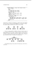
If we draw the shortest path from x to each other vertex in the graph,
then we clearly get no cycles, and we have a spanning tree. Each vertex leads
to a different spanning tree; for example, the following three diagrams show
the shortest path spanning trees for vertices A, B, and E in the example graph
that we’ve been using.
414
CHAPTER 31
The priority-first search solution to this problem is very similar to the
solution for the minimum spanning tree: we build the tree for vertex by
adding, at each step, the vertex on the fringe which is closest to (before,
we added the one closest to the tree). To find which fringe vertex is closest
to we use the array: for each tree vertex k, will be the distance
from that vertex to using the shortest path (which must be comprised of
tree nodes). When k is added to the tree, we update the fringe by going
through k’s adjacency list. For each node t on the list, the shortest distance
to through k from is Thus, the algorithm is trivially
implemented by using this quantity for priority in the priority graph traversal
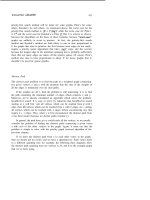
program. The following sequence of diagrams shows the construction of the
shortest path search tree for vertex A in our example.
1
1
2 2
F
WEIGHTED 415
First we visit the closest vertex to A, which is B. Then both C and F are
distance 2 from A, so we visit them next (in whatever order the priority queue
returns them). Then D can be attached at F or at B to get a path of distance
3 to A. (The algorithm attaches it to B because it was put on the tree before

F, so D was already on the fringe when F was put on the tree and F didn’t
provide a shorter path to A.) Finally, E and G are visited. As usual, the tree
is represented by the dad array of father links. The following table shows the
array computed by the priority graph traversal procedure for our example:
ABCDEFG
dad:
ABBFAE
val:
0
1
2 3
4
2 5
Thus the shortest path from A to G has a total weight of 5 (found in the
entry for G) and goes from A to F to E to G (found by tracing backwards
in the dad array, starting at G). Note that the correct operation of this
program depends on the val entry for the root being zero, the convention that
we adopted for sparsepfs.
As before, the priority graph traversal algorithm has a worst-case running
time proportional to (E + V) log V, though a different implementation of the
priority queue can give a algorithm, which is appropriate for dense graphs.
Below, we’ll examine this implementation of priority graph traversal for dense
graphs in full detail. For the shortest path problem, this reduces to a method
discovered by E. Dijkstra in 1956. Though the methods are the same in
essence, we’ll refer to the sparsepfs program of the previous chapter with
priority replaced by [k] + . weight as the “priority-first search solution” to
the shortest paths problem and the adjacency matrix version given below as
“Dijkstra’s algorithm.”
Dense Graphs
As we’ve discussed, when a graph is represented with a adjacency matrix, it is

best to use an unordered array representation for the priority queue in order
to achieve a running time for any priority graph traversal algorithm. That
is, this provides a linear algorithm for the priority first search (and thus the
minimum spanning tree and shortest path problems) for dense graphs.
Specifically, we maintain the priority queue in the array just as in
sparsepfs but we implement the priority queue operations directly rather than
using heaps. First, we adopt the convention that the priority values in the
val array will be negated, so that the sign of a entry tells whether the
corresponding vertex is on the tree or the priority queue. To change the
416 31
priority of a vertex, we simply assign the new priority to the entry for that
vertex. To remove the highest priority vertex, we simply scan through the
array to find the vertex with the largest negative (closest to 0) value
(then complement its entry). After making these mechanical changes to
the sparsepfs program of the previous chapter, we are left with the following
compact program.
procedure densepfs;
var k, min, t: integer;
begin
for to Vdo
begin vaJ[k]:=-unseen; end;
repeat
k:=min;
if vaJ[k]=unseen then :=O;
for to Vdo
if vaJ[t]<O then
begin
if and (vaJ[t]<-priority) then
begin vaJ[t] :=-p dad t] :=k end;
if vaJ[t]>vaJ[min] then min:=t;

end
until
end ;
Note that, the loop to update the priorities and the loop to find the minimum
are combined: each time we remove a vertex from the fringe, we pass through
all the vertices, updating their priority if necessary, and keeping track of the
minimum value found. (Also, note that unseen must be slightly less than
maxint since a value one higher is used as a sentinel to find the minimum,
and the negative of this value must be representable.)
If we use t] for priority in this program, we get Prim’s algorithm
for finding the minimum spanning tree; if we use t] for priority
we get Dijkstra’s algorithm for the shortest path problem. As in Chapter
30, if we include the code to maintain now as the number of vertices so far
searched and use V-now for priority, we get depth-first search; if we use now
we get breadth-first search. This program differs from the sparsepfs program
of Chapter 30 only in the graph representation used (adjacency matrix instead
of adjacency list) and the priority queue implementation (unordered array
WEIGHTED
417
instead of indirect heap). These changes yield a worst-case running time
proportional to as opposed to (E for sparsepfs. That is, the
running time is linear for dense graphs (when E is proportional to but
sparsepfs is likely to be much faster for sparse graphs.
Geometric Problems
Suppose that we are given N points in the plane and we want to find the
shortest set of lines connecting all the points. This is a geometric problem,
called the Euclidean minimum spanning tree problem. It can be solved us-
ing the graph algorithm given above, but it seems clear that the geometry
provides enough extra structure to allow much more efficient algorithms to be
developed.

The way to solve the Euclidean problem using the algorithm given above
is to build a complete graph with N vertices and N(N edges, one
edge connecting each pair of vertices weighted with the distance between the
corresponding points. Then the minimum spanning tree can be found with
the algorithm above for dense graphs in time proportional to
It has been proven that is possible to do better. The point is that the
geometric structure makes most of the edges in the complete graph irrelevant
to the problem, and we can eliminate most of the edges before even starting
to construct the minimum spanning tree. In fact, it has been proven that
the minimum spanning tree is a subset of the graph derived by taking only
the edges from the dual of the Voronoi diagram (see Chapter 28). We know
that this graph has a number of edges proportional to N, and both Kruskal’s
algorithm and the priority-first search method work efficiently on such sparse
graphs. In principle, then, we could compute the Voronoi dual (which takes
time proportional to Nlog N), then run either Kruskal’s algorithm or the
priority-first search method to get a Euclidean minimum spanning tree algo-
rithm which runs in time proportional to N log But writing a program
to compute the Voronoi dual is quite a challenge even for an experienced
programmer.
Another approach which can be used for random point sets is to take
advantage of the distribution of the points to limit the number of edges
included in the graph, as in the grid method used in Chapter 26 for range
searching. If we divide up the plane into squares such that each square
is likely to contain about 5 points, and then include in the graph only the
edges connecting each point to the points in the neighboring squares, then we
are very likely (though not guaranteed) to get all the edges in the minimum
spanning tree, which would mean that Kruskal’s algorithm or the priority-first
search method would efficiently finish the job.
It is interesting to reflect on the relationship between graph and geometric
algorithms brought out by the problem posed in the previous paragraphs. It